
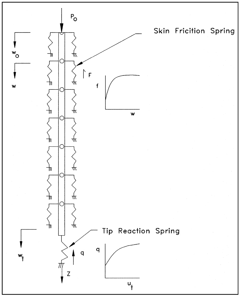
In our last post we discussed the origins and use of these programs to simulate–in forward or inverse analysis mode–the load-settlement characteristics of deep foundations, including driven piles and drilled shafts. In this post we will consider the potential by having these tools at our disposal and some thoughts on how to expand their use and improve their capabilities.
Bearing Capacity and Settlement
I discuss this issue in more detail in my post Driven Pile Design: Axial Loads, General Considerations (and the same considerations apply to bored piles as well.) In that post I state the following:
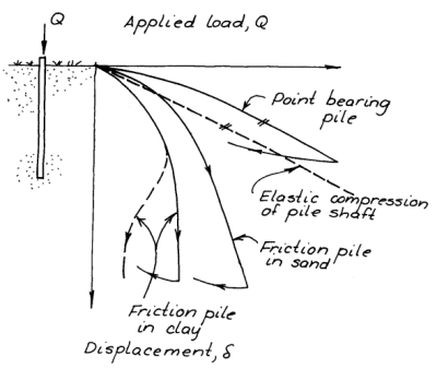
The failure of a deep foundation is progressive, as can be seen at the right. It is very seldom (unless something has gone very wrong somewhere) that pile foundations experience “plunging” (catastrophic) failure, especially if the resistance at the toe is substantial. Put in terms of engineering practice, failure of a deep foundation is most likely to be a service (settlement) failure rather than a strength (bearing capacity) failure. It thus would make sense to design deep foundations based on a settlement criterion. What settlement is acceptable depends upon the application and structure.
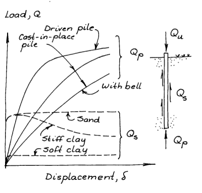
From this, the behaviour of a deep foundation cannot be characterised by a single number. There is a mathematical reason for that. Consider the idealised load-settlement curves below, which include a Davisson method type offset line.
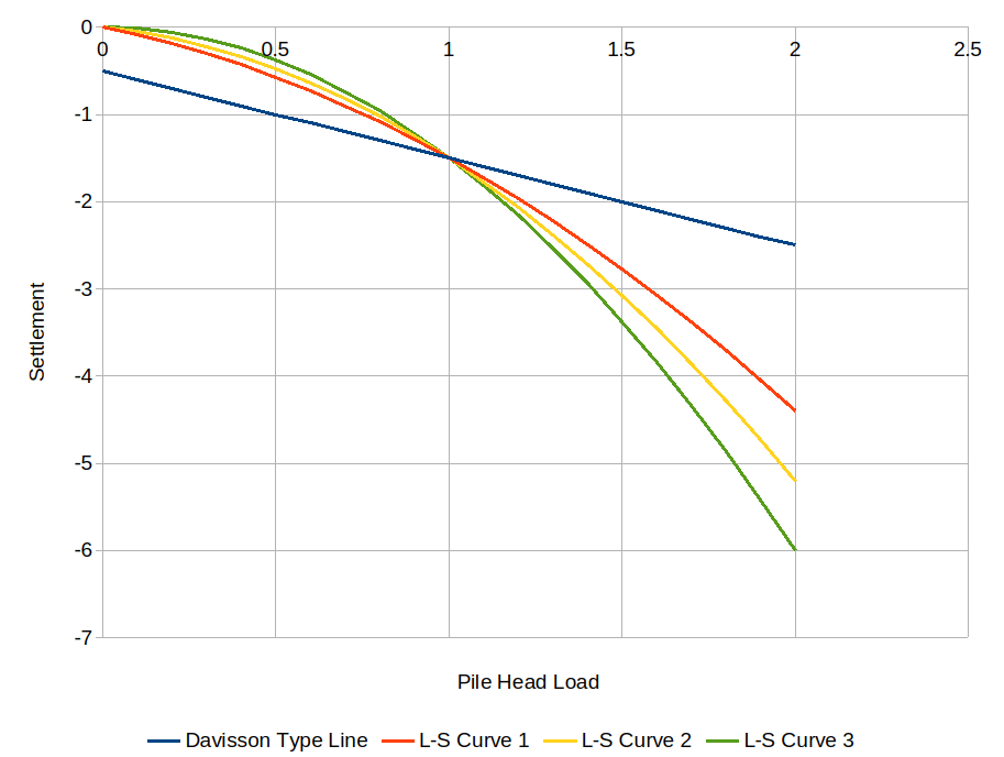
All of the curves (the units were simplified to make the curve constructions easier) pass through the Davisson failure point of (1, -1.5.) But the curves are different, albeit in this case parabolically constructed, and not only that there are an infinite number of them. Thus the load-settlement of a given single-number “bearing capacity” is not unique; the behaviour of the pile under load cannot be adequately characterised by one number.
There are other possible uses for this reality which we will discuss below. Unfortunately the introduction of LRFD has only made the situation worse by formally separating the strength (“bearing capacity”) and service (“settlement”) loads, each with their different load and resistance factor, but each with a single number.
A more sensible way of dealing with this problem would be the following:
- Determine the load-settlement curve(s) for a given project and pile/shaft configuration using software such as APILE.
- Determine the permissible settlement for a foundation depending upon what type of structure supports it. I discuss this on an elementary level in Foundation Design and Analysis: Shallow Foundations, Settlement.
- Adjust the design (or redesign altogether) the foundation until it meets with the requirements of the load. At this point it is legitimate to compare those requirements with whatever static load test capacity method is fashionable in your area, as we would compare both the pile head load and the settlement with those results. (For an overview of Davisson’s method, the most common in the US, visit Driven Pile Design: Static Load Testing and Axial Settlement.)
Since we have the tools for the first analysis, we can proceed with this method with existing technology. The major challenge is to change the design procedures, generally enshrined in the codes or job requirements, and to educate engineers in this methodology.
TZPILE and Resistance/Capacity Distribution
In the last post, we looked at TZPILE and how one could, by matching it to the load-settlement curve, construct a distribution of shaft and toe resistance/capacity along the embedded length of the pile. One is reminded of using the wave equation program to back analyse driven pile results, but these days the most common method is CAPWAP and its progeny. With the numerical methods we have at our disposal, shouldn’t it be possible to construct a distribution of resistance using static data just as CAPWAP does with dynamic?
To start the discussion, take a look at the graph above. Each of the curves (excluding the Davisson type line) represents a different combination of pile configuration and soil resistance/capacity distributions which produce the same Davisson capacity. If we fix the pile configuration, we’re left with soil variations, examples of some of which are at the right. TZPILE enables the user to match this manually. In principle we could automate the process as was done with CAPWAP.
There are, however, a few complications along the way. The math isn’t that complicated but the concepts are not in the daily currency of most practicing geotechnical engineers. I would urge you to take a look at my monograph Least Squares Analysis and Curve Fitting for the basics; it relates the topic to spreadsheet trend lines, which most are familiar with.
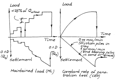
Most static load tests (in the U.S. at least) are performed incrementally, i.e., a load is applied, a settlement is reached, and another load is applied. In many cases the number of loads applied is relatively small. When it’s all done some kind of line is drawn through (or nearly so) the loads to produce a load-settlement curve.
If we do an interpolation, whether it is piecewise linear, Lagrangian or cubic spline, the only thing we can say with confidence is that the curve passes through all of the points. What happens between those point can look good or be accurate but doesn’t have to be either one; it just has to pass through the points.
If we have more or fewer data points than an interpolation would require, we end up looking not for the right solution but the best solution to the problem. That’s where Least Squares Analysis and Curve Fitting comes in, using the ||r||2 norm. (Interestingly CAPWAP uses the ||r||1 norm.) The coefficient of determination R2 gives us a idea as to how good a fit we have, although you need to look at your results to make sure the fit makes sense.
In both cases we cannot use whatever curves between the data points we generate to “fill in” and produce enough data points to effect a one-on-one and onto linear transformation between the static load data and the number of layers the pile might be penetrating into, which is the ideal. With a small number of test loads this could lead to layers and variations in resistance being missed. This is an advantage of CAPWAP; it obtains a large number of data points during driving that in part compensate for the problems of getting a static resistance/capacity out of a dynamic test.
The problem of few load test points is an important one and an obstacle to using a program such as TZPILE on a widespread basis to estimate the load distribution on a deep foundation. If we could increase the number of test points on at least major projects and couple it with a repeatable method of determining the distribution from the load points, we would have yet another source of verification for the load-settlement characteristics of deep foundations.

 vulcanhammer.net
One thought on “APILE and TZPILE: Potential and Challenge”