TAMWAVE 1: Entering Basic Soil and Pile Properties

With a few preliminaries out of the way, we can proceed to discuss the new TAMWAVE routine, which can be found here.

What is TAMWAVE?

TAMWAVE stands for Texas A&M Wave Equation. The TTI wave equation was developed at Texas A&M in the late 1960’s and early 1970’s, and was a successor to Smith’s original wave equation program. In reality this is more than a wave equation program; it is a driven pile analyser which, in addition to the wave equation program, analyses the static performance of a driven pile for both axial and lateral loads. It is not intended to be used on actual projects, but as an educational tool for students. Most of the software in current use is expensive, and predecessors such as SPILE, WEAP87 or COM624 are hard to use (they’re DOS programs) or methodological obsolescence issues. (With WEAP87, there are not as many of those as you might think, but that’s another post…)

Limitations of TAMWAVE

Given that this is an educational tool, there are some significant limitations to TAMWAVE’s capabilities. Some of these are as follows:

Only one type and consistency/density of soil is permitted. However, the phreatic surface can be anywhere between the head and toe of the pile. (If at the toe, the soil is assumed to be dry for the entire length of the pile, an unlikely scenario.)
Piles have uniform cross-section and material for the entire length. Starting in 2010, piles must be picked from a database presented at the start of the routine. This limits the types of piles available, but makes input a lot simpler.
Hammers are likewise limited to air/steam hammers, currently Vulcan and Raymond models. (We may add Conmaco ones, later.) This excludes diesel and hydraulic impact hammers, which simplifies the code considerably.
Both axial and lateral loads are analysed by assuming the soil is either completely cohesionless or cohesive. Unfortunately this is also a limitation of most current driven pile analysis methods as well. Generally speaking, soils are entirely neither, but they’re close enough for current methods. We’ll explore how to deal with this in the STADYN project; for now, we’ll stick with the binary methodology.

Test Case, and Entering the Data

For this series of explanations we’ll use a test case as follows:

12″ concrete pile
100′ long (all piles are groundline in TAMWAVE, so there is no “stick-up” permitted
Water table 50′ below surface
Soil cohesionless or cohesive; in both cases a “medium” soil

Starting with the initial page, the data form looks like this:

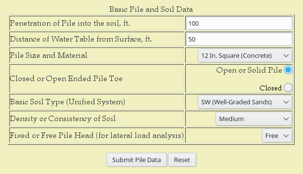
The pile data input is pretty straightforward; the option for closed or open-ended pile toe is only relevant for hollow piles (pipe or concrete cylinder piles.) The soil type is entered using the two-letter Unified system code. This is to accomplish two things:

To make it simple to match the soil description from boring logs, if the problem is stated using one; and
In the case of cohesionless soils, to vary the internal friction angle with the soil type.

Density or consistency choice depends upon whether the soil is cohesionless or cohesive; the following charts (from here) were used for the data:

This slideshow requires JavaScript.

At this point we need to pause and consider something we discussed in our last post: the use of CPT data.

When we attempt to establish soil response to load our ultimate goal is to determine the engineering properties of the soil. Assuming we’re still in a Mohr-Coulomb universe, and setting aside the issue of consolidation settlement, that means three properties: the internal friction angle $\phi$ , the cohesion $c$ , and the unit weight (dry, moist or saturated) $\gamma$ . Ideally we can establish these properties using undisturbed samples in the laboratory. The tricky part comes in obtaining these samples: not only is it expensive, but getting a truly “undisturbed” sample out of the soil is next to impossible, although we can come close. This is why, from the earliest years of geotechnical engineering as a science, we’ve resorted to either tests of disturbed samples (the Atterberg limits are the most prominent of these) or in situ tests such as SPT, CPT or vane shear. In the United States the SPT test has pretty much reigned supreme and is still the most commonly used test, in spite of its manifest limitations and inconsistencies, and appears on many soil boring logs.

Unfortunately most of the “academic” work in pile capacity has centred on the use of CPT results. It was the original idea to essentially convert the SPT results from the charts above to “typical” CPT results and then use these with more contemporary techniques. Unfortunately, in the development of TAMWAVE, it became clear that the results from doing this–especially with the toe response–had problems. Based on this, we decided to drop the use of the artificially generated CPT data and use methods which could be derived from other properties. The reason for this is twofold: the buildup of pore water pressures around the cone tip during insertion made the relationship between $q_c$ and $q_t$ problematic, and this, combined with basic differences in the SPT and CPT methodologies, makes correlating the two not a straightforward proposition. These are discussed in and the geotechnical practitioner would do well to keep this in mind when dealing with the results of either test.

One good thing that resulted from this decision is that we did not have much recourse to the SPT “data” either. We were able to use the “Mohr-Coulomb” triple directly for most of our calculations.

The last piece of data is for lateral piles only: it is whether the head of the pile is “fixed” or “free” for lateral load analysis. The loads themselves will be entered in the next step, which is accomplished by completing the for and pressing the “Submit Pile Data” button.