Author: Don Warrington

SYNOPSIS

Construction vibrations may be harmful to adjacent and remote structures, sensitive instruments and people. Construction vibration sources have a wide range of energy, displacement, velocity and acceleration transmitted on the ground. Effects of different dynamic sources and soil conditions on construction vibrations is analysed. Consequences of construction vibrations are developed in various ways. It is important to assess intolerable vibrations before the beginning of construction activities. Guidelines for preconstruction survey are presented. Pre-construction survey and prediction of anticipated vibrations by IRFP method, monitoring and control of measured vibrations are important steps in preventing intolerable vibration effect.

INTRODUCTION

Implementation of construction projects involve various sources of construction vibrations such as pile driving, dynamic compaction, blasting and operating heavy equipment. These sources generate elastic waves in soil which may adversely affect surrounding buildings. Their effects range from serious disturbance of working conditions for sensitive devices and people, to visible structural damage.

The effect of construction vibrations on surrounding buildings, sensitive devices and people in the urban environment is a significant consideration in obtaining projects approvals from appropriate agencies and authorities. Disruption of some businesses, possible structural damage and annoying people are the problems.

The dynamic effect of construction vibrations on adjacent and remote structures depends on soil deposits at a site and susceptibility ratings of structures. It is likely that intolerable structure vibrations may be induced in close proximity of the driven piles, but foundations settlements resulting from soil vibrations in loose soils may occur at various distances from the source.

There are two opposite extreme opinions regarding vibration effects on surrounding neighborhood. On the one hand according to human perception and psychology, construction vibrations are the causes of all damage in structures, but on the other hand the vibration effect from construction activities is negligible, Oriard (26). Both opinions are wrong and misleading. Proper evaluation of vibration effect is necessary.

It is important to assess the dynamic effect before the beginning of construction activities and at the time of construction. Therefore monitoring construction vibrations have to be started prior to the beginning of construction works at a site and be continued during construction to provide the safety and serviceability of sound and vulnerable structures.

Monitoring and control of construction vibrations were studied by a number of researchers e.g. Attewell and Farmer (1), Barkan (2), Crockett (6), Clough and Chameau (4), Dowding (8), Heckman & Hagerty (13), Lacy and Gould (16), Massarsch (21), Mayne (23), Richart et al. (29), Svinkin (37), Wiss (42), Wood and Theissen (43), Woods (44) and others.

This paper presents some guidelines for preconstruction survey, prediction, measurement, analysis and control of soil and structure vibrations generated by construction activities at a site.

CONSTRUCTION VIBRATIONS

Vibrating, impacting, rotating, and rolling construction equipment is used for soil excavation, modification and improvement. Machinery with dynamic loads and blasting are sources of construction vibrations. The most prevalent powerful sources of construction vibrations are pile driving, dynamic compaction, and blasting. Blasting energy is much larger than energy of other sources of construction vibrations. For example, the energy released by 0.5 kg of TNT is 5400 kJ, Dowding (8). Such energy is 50 to 1000 times the energy transferred to piles during driving and 15 to 80 times the energy transferred to the ground during dynamic compaction of soils, Svinkin (37).

Vibration Classification

Ground vibrations generated by construction sources can be roughly separated into two categories: transient and steady-state vibrations.

The first category includes single event or sequence of transient vibrations and each transient pulse of varying duration is dying away before the next impact occurs. Such vibrations are excited by air, diesel or steam impact pile drivers, by dynamic compaction of loose sand and granular fills, and also by highway and quarry blasts. The dominant frequency of propagating waves from impact sources ranges mostly between 3 Hz and 60 Hz, Svinkin (37).

The vibration records of ground vibrations close to the pile driver are similar to those from forge and drop hammers, Steffens (31). The vibration effects from impact hammers are alike to those from vibrations generated by forge hammers because of comparable energy released and the dominant frequency range.

The second category contains continuous harmonic or some other periodic forms. These forced vibrations are caused by vibratory pile drivers, double acting impact hammers operating at relatively high speeds, and heavy machinery.

Vibratory pile driving equipment is wide spread dynamic source of construction vibrations. The most important characteristics of this machines are frequency with the resultant relationships between dynamic force and eccentric moment. Low frequency machines have vibratory frequency between 5-10 Hz and used mainly for piles with big mass and toe resistance such as concrete and large steel pipe piles. Medium frequency machines have the vibratory frequency range of 10-30 Hz and used with light weight piles such as sheet piles and small pipe piles. High frequency machines operate at frequencies of more than 30 Hz. The major advantage of these machines is their lowered transmission of ground excitation to adjacent structures, Warrington (40).

Vibration Propagation

Sources of construction vibrations generate body (compression and shear) waves and surface waves of which Rayleigh waves are the primary type, Barkan (2) and Richart et al. (29). These waves transmit vibrations through soil medium. Rayleigh waves have the largest practical interest for design engineers because building foundations are placed near the ground surface. In addition, surface waves contain more than 2/3 of the total vibration energy and their peaks particle velocity are major on the velocity records.

Rayleigh waves induce vertical and radial horizontal soil vibrations. In horizontal layering soil medium, a large transverse component of motion could be caused by a second type of surface waves called Love waves rather than other wave types. Waves propagate outward the source in all directions. Spectra of the radial and transverse components of horizontal soil vibrations may have a few maxima and the one corresponding the frequency of the source is not always the largest. In general, faster attenuation of high frequency components is the primary cause of changes of soil vibrations with distance from the source. However, some records can not be explained by this mechanism and the effect of soil strata heterogeneity and uncertainties of the geologic profile should be taken into account, Svinkin (34).

The waves travel outward from the construction source and attenuate in the results of geometrical spreading and material damping. It is common to calculate displacement amplitude reduction of the Rayleigh wave between two points at distances r₁ and r₂ from the source as (r₁/r₂)^0.5 with a factor exp[-α(r₁-r₂)] where α is the coefficient of attenuation, Golitsin (10). However, there are certain difficulties in determination of the coefficient, α, for ground vibrations from construction and industrial sources. This coefficient could be inadequate for different distances between points of measurements. On account of wave refraction and reflection from boundaries of diverse soil layers, an arbitrary arrangement of geophones at a site can yield incoherent results of ground vibration measurements because waveforms measured at arbitrary locations at the site might represent different soil layers, Svinkin (37).

Besides, the coefficient, α, depends on the soil resistance to pile penetration. During hard driving, these coefficients tend to be higher than those where hard driving is not encountered. According to experimental data from Clough and Chameau (4), the coefficients, α, were 1.3-2.5 times greater for hard driving than those for normal driving.

A scaled-distance approach, Wiss (42) and Woods (44), uses relationship between energy, W, of source and surface distance, D, where velocity, v, is calculated as (D/W^0.5)^-n where the value of ‘n’ yields a slope in a log-log plot between 1 and 2. The modified scaled-distance approach provides calculation of the peak particle velocity (PPV) of ground vibrations as a function of the source velocity, Svinkin (35).

Mayne (23) suggested for dynamic compaction a relationship between the impact velocity of a free falling weight and PPV of ground vibrations as PPV= 0.2(2gH)^0.5(d/r₀)^-1.7 where g = gravitational constant, H = falling height, d/r₀ = distance normalized to the weight radius.

Empirical equations employed for assessment of expected soil vibrations from construction and industrial sources usually only allow calculation of a vertical peak amplitude of vibrations and not always with sufficient accuracy. These equations cannot incorporate specific differences of soil conditions at each site because heterogeneity and spatial variation of soil properties strongly affect characteristics of propagated waves in soil from construction and industrial vibration sources.

A new Impulse Response Function Prediction method (IRFP) has been originated by Svinkin (34, 36) for determining complete time domain records on existing soils, structures and equipment prior to installation of construction and industrial vibration sources. The IRFP method has significant advantages in comparison with empirical equations and analytical procedures.

Vibration Damage and Disturbance Criteria

A number of attempts have been made to connect vibration parameters (displacement, velocity and acceleration) with observed human annoying, disturbances of sensitive devices, and structural damage, for example, Crandell (5), Medearis (24), Nichols et al. (25), Raush (28), Siskind et al. (30) and others. Richart et al. (29) demonstrated some results of such studies in graphical form for structure and machine vibration limits combined with human perception limits.

It was found that structural damage could be well correlated with the peak particle velocity (PPV) of structure vibrations. The same criterion for structural damage of residential buildings was set at 50 mm/s peak particle velocity in the frequency range of 3-100 Hz, Nichols et al. (25). For commercial and engineered structures, Wiss (41) suggested to use a conservative limit of 100 mm/s.

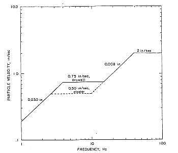
Building damage occurs in the result of combined influence of structure vibration displacement, velocity, acceleration and frequency. The necessity to take into account the vibration frequency to assess the vibration effect on structures was underlined in a number of publications, for example, Dowding (7, 8), Medearis (24), Siskind et al. (30), Svinkin (32) and others. Intensive studies of residential structural damage in connection with measured displacement and velocity was made by the U.S. Bureau of Mines, Siskind (30). As the results, a set of criteria was developed for the frequency range of 1-100 Hz, involving both displacement and velocity, Figure 1.

The peak particle velocity is the parameter most commonly used to evaluate the effect of construction vibrations on structure. However, other vibration parameters should be used in assessment of vibration effects as well. So Figure 1 shows the importance of displacement limits to evaluate structural damage. Displacement of 0.1 mm, and acceleration of 2.5 m/s², not velocity, are vibration limits for computing systems, Boyle (3).

There are simple mathematical relationships between peaks of displacement, velocity and acceleration. Displacement calculations from velocity records are correct, but analogous acceleration calculations do not always yield proper results because velocity measurement cannot detect high frequency components of ground vibrations. Accelerometers and geophones have the opposite principles for vibration measurements. If acceleration limits are available for sensitive devices or foundation settlements, acceleration must be measured in parallel to velocity measurements. For example, Clough and Chameau (4) made acceleration and velocity measurements at the same time. One more important point is to use devices with proper calibration curves. Otherwise it is possible to receive misleading results.

SURVEY OF CASE STUDIES

There are numerous publications regarding vibration effects from construction operations. Several references are presented in the introduction section of this paper. In this section, an attempt was made to analyse obtained results and assess contribution of different factors on construction vibrations.

Source Effect on Ground Vibrations

Pile Type. In general, piles being driven as displacement piles generate the greatest ground vibrations, e.g. Woods (44), Svinkin et al. (38) and others. However, there effects are varied and depend on pile cross-section shape and soil conditions. The more pronounced effects of displacement piles on ground vibrations occurs predominantly at distances less than 10 m from pile driving,

A pile shape may affect ground vibrations around the driven pile. Martin (20) found that driving of sheet piles do not generate large horizontal vibrations in perpendicular direction to the line of the sheet piles.

Pile impedance is a significant factor in the transfer of dynamic longitudinal force into the pile and from the pile into the surrounding soil. The greater the pile impedance, the greater the pile capacity and the greater the dynamic force that can be transferred to the ground. However, pile impedance affects the intensity of ground vibrations in two opposite ways at the same time. On the one hand, increasing pile impedance increases the force transmitted to the pile and surrounding ground, but on the other hand, increasing pile impedance decreases the peak particle velocity of pile and ground vibrations. An increase of hammer energy magnifies ground vibrations until the pile impedance allows to increase the force transmitted to the pile and the surrounding soil. The impedance affects in opposite ways the force and the velocity transmitted to the ground and therefore the pile impedance effect on the intensity of ground vibrations is not obvious. Pile impedance cannot be always used as a predictor of intensity of ground vibrations, Svinkin et al. (38).

Soil Resistance and Pile Length. During driving, the various soil resistances to pile penetration are developing as the pile penetration depth is increasing. Pile-soil load transfer is realized by means of both concentrated loads from the pile toe and distributed loads generated along the pile shaft. Generally speaking, dynamic loads transferred from the pile to the ground should be increasing with augmentation of a pile penetration depth. However, this does not always occur. Accumulated experience in pile driving shows that the intensity of ground vibrations is mostly independent of the pile penetration depth and depends on soil properties, for example, Clough and Chamean (4), Holloway et al. (15), Svinkin et al. (38) and others.

In soils with a low penetration resistance such as loose fill, peat or silt, a large portion of the hammer energy is used in overcoming soil friction and thereby moving piles down. Therefore less energy is transmitted for generating ground vibrations in comparison with pile driving in soil with a high penetration resistance. The high blow count resulted in increased ground vibrations at the pile penetration depth approximately between 4-8 m below the ground surface but did not effect ground vibrations at the greater depth. These results were obtained from driving of concrete, steel shell and H piles and also of sheet piles.

Dynamic Compaction. For dynamic compaction of loose sands and granular fills, large and heavy steel or concrete blocks weighing typically 49.1-137.3 kN are usually dropped from heights of up to 30 m, Hayward Baker (12). The size of weights could be larger at some construction sites. The maximum falling weight found in publications was 397.3 kN, Gambin (9).

The wide range of impact loads on the ground determines a wide range of ground vibrations. Vibration levels increase as the treated field becomes densified. A maximum level of particle velocity might be achieved after one or two passes of heavy tamping. It is necessary to point out that localized liquefaction may occur around the contact area of impact, Mayne (22).

Dynamic loads on the ground induce elastic waves in the soil medium and these waves are transmitted through the soil in all directions. The spectra of soil vibrations excited by impacts show a few maximums with the dominant frequency of the surface wave. Actually, these frequencies are the natural frequencies of the soil layers and the values obtained do not practically depend on conditions at the contact area where impacts are made directly on the soil. In general, soil profiles are nonlinear systems and the dominant frequency of soil profiles depends on the applied impact. Nevertheless, over a certain range, the system behavior may be linear and if the system is restricted to this range it is possible to safely use the linear approach. However if sizes of falling weights are considerably different, such impacts on the same contact area might generate surface waves with different dominant frequencies, Svinkin (33, 34).

Blasting. Blasting energies are much larger than energies of other sources of construction vibrations. Blast design depends on the large number of factors and is aimed to enhance blasting productivity and diminish generated ground vibrations without increasing the cost. The following describes effects of different factors on ground vibrations, Nicholls et al. (25), Dowding (8) and OZA Inspections (27).

Explosive type and weight, delay-timing variations, size and number of holes, distance between holes and rows, method and direction of blast initiation, geology and overburden are the most important causes which effect ground vibrations. The explosive types affect ground motion through detonation velocities of explosives and a square root of the charge weight. Microsecond-delayed blasts are used for reduction of PPV of ground vibrations which are connected with the maximum charge weight detonated per delay. A choice of the proper delay is not a simple problem. Wave propagation might differ with direction if there is geologic complexity. The effect of overburden manifests itself in attenuation of high-frequency components of ground motion.

Energy of Dynamic Sources. The energy of construction sources is important source property which effects intensity of surface waves, e.g. Attewell and Farmer (1), Mayne (23), Wiss (42), Woods (44) and others. In general, ground vibration level increases if the source energy increase. However the energy of source is not always the dominant factor in determination of the intensity of ground vibrations. The following case studies shows that influence of other factors should be considered.

The effect of energy level of dynamic compaction on PPV of ground vibrations at different distances from the source was studied by Mayne (23). It was revealed that the exponent term for energy of the source, W, decreases with distance away from the point of impact. At distances of 6.1, 15.25, and 30.5 m, the observed effect of energy level was ^0.6, ^0.5, and ^0.4, respectively, as determined from linear regression analysis of obtained data.

Martin (20) reported similarity of PPV of vertical ground vibrations observed for displacement piling on peat and corresponding PPV observed for sheet piling on silt and clay. Although the impact energy of the hammer used for driving of close-ended steel pipes was in ten times the energy of the hammer used for sheet piling, the intensity of vertical ground vibrations was similar at the compared construction sites. The minor reason of these results was explained by differences in the geometry of the piles. The displacement pile had a circular section and the energy transmitted from this pile to the ground was shared between vertical and two horizontal components of ground vibrations. The sheet pile had a ‘U’ shaped section and driving of this pile produced predominantly vertical ground vibrations. The major reason for the comparatively low level of vertical vibrations from displacement piling operation was the low penetration resistance of the peat. A large portion of the energy transferred to the pile was absorbed in moving the pile through the peat.

Dowding (8) made comparison of ground vibrations induced by pile driving with a diesel hammer and by Franki pile driving and revealed that the latter developed two times more energy but induced smaller ground vibrations at the same distances from the sources. Perhaps the cause of this phenomenon was a higher attenuation of surface waves in the loose soil deposits where Franki piles were driven. This observation underlines the significance of soil contribution to the formation of ground vibrations.

Soil Effect on Vibrations Propagation

Distance from Sources. Waves travel in all directions from the source of vibrations forming a series of fairly harmonic waves with the dominant frequency equal or close to the frequency of the source. Higher frequencies being attenuated faster than lower frequencies with distance from the source. However, the soil medium does not consistently play the role of a low-pass filter and ground vibrations with higher frequencies and amplitudes may arise after certain vibration attenuation.

The inherent spacial variations of soil properties are not always readily identifiable by routine boring, sampling, and testing. For instance, Hammond (11) reported a case history of the influence of heterogeneity in soil strata on soil and building vibrations at the site where a foundation was installed for a forge hammer with a falling weight of 75.8 kN. The dominant frequency of propagated waves was 22.0 Hz to the west of the hammer foundation, while, at the same time, in opposite direction to the east of the source, the dominant frequency was 10.0 Hz. In another interesting case, Svinkin (34), forge hammer foundation vibrations with a frequency of 14.0 Hz excited soil vibrations with a similar dominant frequency except at one location where the dominant frequency was 25.0 Hz with enhanced amplitudes.

Soft and Stiff Soils. Attenuation of surface waves with distance from the source is important for reduction of ground vibrations. Clough and Chameau (4), Wiss (42) and Wood and Theissen (43) made intensive measurements of ground vibrations from construction sources and revealed that values of geometric and material damping are higher in soft soils than those in denser, firmer soils. Moreover, PPVs of ground vibrations tend to increase as soil materials become more dense with the number of blows, Mayne (22). Nevertheless, there is an opposite point of view. Taniguchi and Okada (38) described a case where soft ground was improved to depth of 12 m by means of the lime pile method. As a result, the acceleration at the ground surface decreased to 10-60 % in the frequency range less than 10 Hz. Indeed, various soil conditions require different solutions to diminish ground vibrations.

Martin (20) reported results of measured ground vibrations which had been induced by Love waves. A closed-ended pipe pile was being driven by a drop hammer into the soft clay to the depth of about 8 m and then into the gravel layer. When the pile reached the gravel level, PPV of transverse ground vibrations increased two times but PPV of vertical and radial motion were almost the same. The large transverse vibrations were a Love surface wave. Similar large transverse ground motion was recorded by Clough and Chameau (4) during driving sheet piles through the rubble layer by an ICE Model vibratory hammer at an operated fixed frequency of 1,100 rpm.

CONSEQUENCES OF CONSTRUCTION VIBRATIONS

Vibrations transmitted through the ground during construction operations may annoy people and detrimentally effect structures and sensitive devices.

Construction vibrations effect structures in two major ways. Those vibrations may produce direct damage to structures and make damage due to vibration-induced settlement.

Structure Vibrations. Structure vibrations depend on soil-structure interaction which determines a structure response to the ground excitations. Structure vibrations measured from construction operations vary in a wide range of frequency content and intensity.

Case studies made by Wood and Theissen (43) included ten projects with vibration levels measured in buried structures and buildings supported on piles at soft soil sites and on spread footings at firm soil sites. It was concluded that vibratory hammers of about 23 kg-m eccentric moment or impact hammers of about 94 kJ rated energy with a weight of striking parts of 43.3 kN operating immediately adjacent to unreinforced brick or reinforced concrete structures in poor conditions may be in some degree dangerous for building. Similar construction sources operating immediately adjacent to reinforced concrete structures in good conditions will probably do not produce dangerous structure stresses. Results obtained by Mallard and Bastow (19) and Martin (20) showed that vibrations of light floors are larger and concrete floors are smaller than ground vibrations.

The proximity of the frequency of soil vibrations to one of the structures natural frequencies may generate the condition of resonance in the building. Continuous forced vibrations produced by vibratory hammers have potential to set up resonant vibrations in certain building structures. Moreover transient vibrations might trigger resonant vibrations as well. Levin (17) found that 3-4 cycles of ground vibrations could generate the condition of resonance in the building. Rausch (28) described a case history where intolerable vibrations occurred in an administrative building located 200 m from the foundation of a forge hammer with a falling weight of 14.7 kN. This weight was considerably less than that in the described above case, Wood and Theissen (43), but obviously the condition of resonance played the major role.

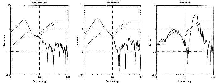
The damage criteria in Figure 1 are used as a threshold level, but it does not mean that exceeding this level immediately entail some structural damage. For example, ground vibrations measured nearby the school building located at distance of 24.4 m from a construction blast are shown in Figure 2, OZA Inspections (27). It can be seen that PPV of vertical, radial and transverse ground vibrations were higher of the threshold levels for the wide frequency range. Such vibrations did not result damage of one story brick school building supported on concrete foundations.

One more important comment. The damage criteria displayed in Figure 1 do not make distinction of type, age and conditions of structures and foundations. Probably more objective and informative damage criteria are a subject for future research.

Crockett (6) and Dowding (8) suggested to take into account the accumulated effect of repeated dynamic loads, for example from production pile driving. This approach is especially important for historical and old buildings.

On the basis of probabilistic analysis of a numerous published data, Siskind et al. (30) made a damage description for Uniform Classification. The three damage categories included the following. Threshold: loosening of paint, small plaster cracks at joints between construction elements. Minor: lengthening of old cracks, loosening and falling of plaster, cracks in masonry around openings near partitions, hairline to 3 mm cracks, fall of loose mortal. Major: cracks of several millimetres in walls, rupture of opening vaults, structural weakening, fall of masonry, load support ability affected. This classification can be useful in assessment of structural damage from construction vibrations.

Settlements Induced by Vibrations. Vibrations may change properties of loose sands saturated with water. This physical phenomenon produces settlement of the ground around the pile and building foundations. Lacy and Gould (16) collected 19 reported cases with different settlements of sands caused by pile driving, described a few approaches to calculate ground settlement, and underlined problems in calculation of settlement of loose sand during pile driving.

It is not clear what vibration parameter and its value should be considered as a trigger of a liquefaction phenomenon of sand. Lacy and Gould (16) consider PPV of ground vibrations of 2.5 mm/sec as a threshold of possible significant settlements at vulnerable sites. Clough and Chameau (4) and Lukas and Gill (18) used an acceleration for assessment of ground and foundation settlement. Barkan (2) reported an important role of the static pressure on the soil for dynamic settlement of a foundation. Therefore different criteria should be taken into consideration in assessment of potential liquefaction problem.

Human Responses. Human perception of vibrations is subjective and human response to arisen vibrations may have false reasoning. Therefore contractor have to provide proper public relations to inform residents regarding possible negative effects of construction vibrations.

MITIGATION OF VIBRATION PROBLEMS

A pre-construction survey is the first step in the control of construction vibrations to ensure safety and serviceability of adjacent structures and/or distant structures with sensitive equipment like hospital facilities and offices with precision instruments. According to pile driving practice, construction vibrations may cause direct damage to structures at a distance about of one pile length from the driven pile. However, there is no single opinion regarding the maximum radius of a preconstruction survey area with buildings surrounding a construction site. Dowding (8) suggested a radius of 120 m of a construction activities, or out to a distance at which vibrations of 2 mm/s occur. Woods (44) considered distances of as much as 400 m to be surveyed to identify settlement damage hazards. Obviously, a radius of the area of preconstruction survey is various and depends on building condition and utilization.

The preconstruction survey includes a few steps of site investigations.

Inspect present conditions of surrounding buildings.

Perform damage susceptibility study to establish vibration control limits.

Measure vibration background at the area under investigation.

Assess problems such as cracking of building or foundation failure.

First of all a preliminary desk study of a layout of the area for a preconstruction inspection and a site walk-over observation should be made. Existing cracks found in buildings have to be marked. It is necessary to distinguish cosmetic and structural cracks. Most attention should be paid to cracks in the structures themselves. The width of cracks should be measured with a proper ruler. Determining the cause of cracking is important to predict lengthening and dilatation of old cracks under the vibration effect of pile driving.

For assessment of the dynamic effect on surrounding structures it is necessary to take into account the thresholds of damage, cracking and perception. Buildings inspected under the contract requirements are commonly classified depending on structure susceptibility to cracking and proximity of structures to pile driving operations.

Structure susceptibility is usually related to the threshold of cosmetic cracking, Dowding (7), and depends on a degree of degradation of the building structural and nonstructural systems. Apparently this terminology should be used in the broad sense as susceptibility of the building-soil system depending on degradation of building systems, utilization of buildings and soil conditions. It is important for certain cases. For example, a building, located in the proximity of the driven piles, identified as having low susceptibility and built on liquefiable soils might have substantially larger deformations than a building identified as having high susceptibility but erected on non-liquefiable soils at long distance from the driven piles. Certainly, for some sites only the threshold of cosmetic cracking could be sufficient.

Measurement of a vibration background at soil and buildings with sensitive equipment and/or computerized technology should be a part of the preconstruction survey. The vibration measurement might reveal microvibrations and vibrations induced by industrial machinery located nearby. A waveform recorder has to be used for these measurements.

Assessment of the dynamic effect of construction operations on surrounding structures can be made on the basis of prediction, monitoring and control of soil and structures vibrations from pile driving.

CONCLUSIONS

Construction operations involve various sources of vibrations such as pile driving, dynamic compaction, blasting and operating heavy equipment. Construction work often creates problems of disruption of some businesses, annoying people and possible structural damage.

Dynamic loads transmitted to the ground change in a wide range of frequency content and intensity and generate elastic waves in soil medium.

Empirical equations provide only calculation of a vertical amplitude of ground vibrations and not always with sufficient accuracy.

The impulse response function prediction method (IRFP) has obvious advantages in predicting time domain ground and structure vibrations prior to the beginning of construction activities.

Parameters of dynamic sources and soil conditions effect soil and structure vibrations. Various factors such as pile type and length, soil resistance, specific peculiarities of dynamic compaction and blasting should be considered in analysis of vibration effects.

The preconstruction survey should be made to ensure safety and serviceability of adjacent structures and/or remote structures with sensitive equipment like hospital facilities and offices with precision instruments.

It is important to assess the dynamic effect before the beginning of construction activities and at the time of construction. Therefore monitoring construction vibrations have to be started prior to the beginning of construction work at a site and be continued during construction to provide the safety and serviceability of sound and vulnerable structures.

REFERENCES:

1. ATTEWELL, P.B. and FARMER, I.W. Attenuation of ground vibrations from piles. Ground Engineering, 1973, Vol. 6(4), pp. 26-29.

2. BARKAN, D.D. Dynamics of bases and foundations. McGraw Hill Co., New York, 1962.

3. BOYLE, S. The effect of piling operations in the vicinity of computing systems. Ground Engineering, 1990, June, 23-27.

4. CLOUGH, G.W. and CHAMEAU, J.L. Measured effects of vibratory sheetpile driving. Journal of the Geotechnical Engineering Division, ASCE, 1980, Vol. 106, No. GT10, 1081-1099.

5. CRANDELL, F.J. Ground vibration due to blasting and its effects upon structures. Journal of the Boston Society of Civil Engineers Section/ASCE, 1949, Vol. 3, 222-245.

6. CROCKETT, J.H.A. Piling vibrations and structural fatigue. Recent Developments in the Design and Construction of Piles, The Institution of Civil Engineers, London, 1980, 305-320.

7. DOWDING, C.H. Ground-structure response to blasting vibrations. Proceedings of the 14th Annual meeting, Society of Engineering Science, 1977, 1085-1093.

8. DOWDING, C.H. Construction Vibrations. Prentice Hall, Upper Saddle River, 1996.

9. GAMBIN, M.P. Menard Dynamic Compaction. Proceedings of ASCE National Capital Section Seminar on Ground Reinforcement, George Washington University, Washington, D.C., January 1979.

10. GOLITSIN, B.B. On dispersion and attenuation of seismic surface waves (in German). Russian Academy of Science News, 1912, Vol. 6, No. 2.

11. HAMMOND, R.E.R. Vibration-controlled foundations at Salten. Iron and Steel, 1959, Vol.32, No.3.

12. HAYWARD BAKER. Dynamic Compaction – Information, Odenton, Maryland, 1999.

13. HECKMAN, W.S. and HAGERTY, D.J. Vibrations associated with pile driving. American Society of Civil Engineers, ASCE Journal of the Construction Division, 1978, Vol. 104, No. CO4, pp. 385-394.

14. HEISEY, J.S., STOKOE, K.H.II, and MEYER, A.H. Moduli of pavement systems from spectral analysis of surface waves. Research Record No. 852, Transportation Research Board, 1982, 22-31.

15. HOLLOWAY, D.M., MORIWAKI, Y, DEMSLY, E., MOORE, B.H. & PEREZ, J.Y. 1980. Field study of pile driving effects on nearby structures, Special Technical Publication, Minimizing Detrimental Construction Vibrations, Preprint 80-175, New York, 1980, 63-100.

16. LACY, H.S. and GOULD, J.P. Settlement from pile driving in sands. American Society of Civil Engineers, Proceedings of ASCE Symposium on Vibration Problems in Geotechnical Engineering, Detroit, Michigan, G. Gazetas and E.T. Selig, Editors, 1985, 152-173.

17. LEVIN, G.E. Dynamic influence of drop hammer foundations on surrounding structures (in Russian). Proceedings of the Second Conference on Dynamics of Bases and Foundations, 1969, 147-152. Moscow: NIIOSP

18. LUKAS, R.G. and GILL, S.A. Ground movement from piling vibrations. Piling: European practice and worldwide trends, Thomas Telford, London, 1992, 163-169.

19. MALLARD, D.J. and BASTOW, P. Some observations on the vibrations caused by pile driving. Recent Developments in the Design and Construction of Piles, The Institution of Civil Engineers, London, 1980, 261-284.

20. MARTIN, D. Ground vibrations from impact pile driving. Transport and Road Research Laboratory, Supplementary Report 544, Crowthorne, England, 1980.

21. MASSARSCH, K.R. Keynote lecture: Static and dynamic soil displacements caused by pile driving. Proceedings of the Fourth International Conference on the Application of Stress-Wave Theory to Piles, F.B.J. Barends, Editor, The Hague, The Netherlands, 1992, 15-24.

22. MAYNE, P.W. Ground response to dynamic compaction. Journal of Geotechnical Engineering, ASCE, 1984, Vol. 110, No. 6, 757-774.

23. MAYNE, P.W. Ground vibrations during dynamic compaction. American Society of Civil Engineers, Proceedings of ASCE Symposium on Vibration Problems in Geotechnical Engineering, Detroit, Michigan, G. Gazetas and E.T. Selig, Editors, 1985, 247-265.

24. MEDEARIS, K. Development of rational damage criteria for low-rise structures subjected to blasting vibration. Proceedings of the 18th Symposium on Rock Mechanics, 1977.

25. NICHOLLS, H.R., JOHNSON, C.F., and DUVALL, W.I. Blasting vibrations and their effects on structures. U.S. Department of Interior, Bureau of Mines Bulletin 656, 1971.

26. ORIAD, L.L. The effects of vibrations and Environmental forces. International Society of Explosives Engineers, Cleveland, 1999.

27. OZA Inspections Ltd. Construction vibrations and noise monitoring – Reports 1990-1999, Lewiston, New York.

28. RAUSCH, E. Maschinen fundamente (in German), VDI-Verlag, Dusseldorf, Germany, 1950.

29. RICHART, F.E., HALL, J.R. and WOODS, R.D. Vibrations of soils and foundations. Prentice-Hall, Inc., Englewood Cliffs, New Jersey, 1970, 414.

30. SISKIND, D.E., STAGG, M.S., KOPP, J.W., and DOWDING, C.H. Structure response and damage produced by ground vibrations from surface blasting. Report of Investigations 8507, U.S. Bureau of Mines, Washington, D.C., 1980.

31. STEFFENS, R.J. Structural vibration and damage. Building Research Establishment Report, HMSO, 1974.

32. SVINKIN, M.R. Pile driving induced vibrations as a source of industrial seismology. Proceedings of the 4th International Conference on the Application of Stress-Wave Theory to Piles, The Hague, The Netherlands, F.B.J. Barends, Editor, A.A. Balkema Publishers, 1992, 167-174.

33. SVINKIN, M.R. Discussion of ‘Impact of weight falling onto the ground’ by Roesset, J.M. et al., Journal of Geotechnical Engineering, ASCE, 1996, Vol. 122, No. 5, 414-415.

34. SVINKIN, M.R. Overcoming soil uncertainty in prediction of construction and industrial vibrations. American Society of Civil Engineers, ASCE, Proceedings of Uncertainty in the Geologic Environment: From theory to Practice, Geotechnical Special Publications No. 58, C.D. Shackelford, P. Nelson, and M.J.S. Roth, Editors, 1996, Vol. 2, 1178-1194.

35. SVINKIN M.R. Velocity-impedance-energy relationships for driven piles. Proceedings of the Fifth International Conference on the Application of Stress-Wave Theory to Piles, Orlando, F. Townsend, M. Hussein and M. McVay, Editors, 1996, 870-890.

36. SVINKIN, M.R. Numerical methods with experimental soil response in predicting vibrations from dynamic sources. Proceedings of the Ninth International Conference of International Association for Computer Methods and Advances in Geomechanics, Wuhan, China, J.-X. Yuan, Editor, A.A. Balkema Publishers, 1997, Vol. 3, 2263-2268.

37. SVINKIN, M.R. Prediction and calculation of construction vibrations. DFI 24th Annual Members’ Conference, Decades of Technology – Advancing into the Future, 1999, 53-69.

38. SVINKIN, M.R., ROTH, B.C., and HANNEN, W.R. The effect of pile impedance on energy transfer to pile and ground vibrations. Proceedings of the Sixth International Conference on the Application of Stress-Wave Theory to Piles, Sao Paulo, Brazil, 2000.

39. TANIGUCHI, E. and OKADA, S. Reduction of ground vibrations by improving soft ground. Soil and Foundations, JSSMFE, 1981, Vol. 21, No. 2, 99-113.

40. WARRINGTON, D.C., 1992. Vibratory and impact-vibration pile driving equipment. Pile Buck, Inc., Second October Issue, 1992, 2A-28A.

41. WISS, J.F. Effect of blasting vibrations on buildings and people. Civil Engineering, ASCE, 1968, July, 46-48.

42. WISS, J.F. Construction vibrations: State-of-the-Art. American Society of Civil Engineers, ASCE Journal of Geotechnical Engineering, 1981, Vol. 107, No. GT2, 167-181.

43. WOOD, W.C and THEISSEN, J.R. Variations in adjacent structures due to pile driving. Proceedings of the GEOPILE Conference, San Francisco, 1982, 83-107.

44. WOODS R.D. Dynamic effects of pile installations on adjacent structures. Synthesis Report, National Cooperative Highway Research Program NCHRP Synthesis 253, Washington, D.C., 1997.

M.R. SVINKIN
Consulting Engineer, Cleveland, OH

ABSTRACT: Reliability of dynamic methods for determination of pile capacity is particularly important for piles driven in clayey soils. This paper shows the conditions for proper comparison of static load test and dynamic testing results, analyses the causes of erroneous prediction of pile capacities computed by wave equation analysis, and demonstrates that application of a variable damping coefficient can improve the reliability of wave equation solutions.

1 INTRODUCTION The capacity of a driven pile changes with time after installation. Soil consolidation and dissipation of excess pore pressure generated during pile driving in the soil-pile interface zone are usually accompanied by an increase in pile capacity. In clayey soils, Seed & Reese (1955) and also Thorburn & Rigden (1980) found an increase in pile capacity (also called setup factor) of up to 6 times over a period of 30 days. In clays, Svinkin et al. (1994) reported the range of setup factors between 4.5 and 11.4 for a period of 22-35 days. Therefore, the assessment of the actual pile capacity after the completion of driving is important for reliable and economic design of pile foundations. In practice, pile capacity is verified by static and/or dynamic tests. Also, there are predictive numerical computations of the pile capacity such as dynamic formulas and wave equation analysis. This paper considers some aspects of verification of dynamic testing results and proposes a variable damping coefficient as a way to increase accuracy and reliability of wave equation analysis in predicting pile capacity in clayey soils. 2 ADEQUACY OF STATIC AND DYNAMIC TESTS It is common in practice to predict the pile capacity by static analysis based on results of in-situ and/or laboratory soil property tests. The static axial load test (SLT) is traditionally used to confirm the computed soil resistance and to determine the service load that can be supported by a pile. The procedure consists of driving the pile to the design depth and applying a series of static loads. Over the past 30 years, Dr. G.G. Goble and associates pioneered the development of pile capacity calculations from measured force and velocity at the pile head. Dynamic pile testing has become wide spread as a replacement for or supplement to SLT because of its inherent savings in cost and time. Dynamic testing methods are described in Goble et al.(1980), Rausche et al. (1985), Hannigan (1990), Holeyman (1992). These methods allow monitoring pile driving and restrikes, identifying problems during driving, and providing inspection of driving quality for many kinds of piles. To obtain reliable ultimate resistance, it is necessary that the long term pile capacity be fully mobilized. Dynamic testing methods can determine static capacity at the time of testing, at the end of driving or at restrikes. This is a substantial advantage, because dynamic tests can be easily repeated and, consequently, there is an opportunity to obtain pile capacity as a function of time as well as pile embedment. In spite of a number of problems with implementation of the SLT and interpretation of the ultimate pile capacity, the SLT is considered as the most reliable method to determine pile capacity (Poulos & Davis 1980; Fellenius 1980; Edde & Fellenius 1990). Because dynamic testing (DT) is often used to replace the SLT, it is important to ascertain the adequacy of both SLT and DT. Static and dynamic methods to determine the ultimate pile capacity are based on different physical principles, but when both tests are performed on the same pile, they can yield results which together present the pile capacity as a function of time (Svinkin et al. 1994). For different piles driven in clayey soils, time dependent pile capacity can be expressed by relationships such as a linear equation in a logarithmic time scale (Scov & Denver 1988). By way of illustration, the pile capacities from SLT and DT are shown in Figure 1 and Table 1 for a 610 mm square prestressed concrete pile with a 305 mm diameter hollow center. Setup factors were 3.42, 5.73, 6.25 and 6.90 for restrikes 1, 2, 3 and SLT, respectively, Table 1. The depth of pile penetration was 24.4 m, and the soil consisted of about 25.6 m of mainly gray clays followed by a bearing layer of silty sand. The water table was at the ground surface. A Delmag 46-13 hammer was employed for both initial driving and restrikes (RSTR). Driving data are shown in Table 2. In Figure 1, variable t is the time after the end of initial driving (EOID) and for this example t0=1 is the time elapsed after EOID from which an increase in pile capacity is linear on a logarithmic time scale (to=time from EOID to the first restrike in days). SLT and DT present different ways in determining pile capacity at various times after pile installation, but two principal conditions have to be the same for both kinds of tests. It is absolutely necessary that static and dynamic capacities are being compared only at the same time of testing of both SLT and DT. Moreover, the ultimate pile capacity can be obtained by SLT only if SLT provides the fully mobilized pile capacity similarly to DT. The adequacy of SLT and DT have to be confirmed by proper correlation of dynamic methods. It is known that dynamic testing methods yield pile capacity only for the time of testing (Rausche et al. 1985, Likins et al. 1988). Some published data demonstrate comparison of SLT and DT results without taking into account the time between different tests (Rausche et al. 1985, Denver & Skov 1988, Hunt & Baker 1988, Hannigan 1990, Paikowsky & Chernauskas 1992, Lee et al. 1996, Liu et al. 1996). Such a comparison is invalid for piles driven in clayey soils because the results of DT do not correspond to those of SLT i.e. soil consolidation is taken into account for DT and is not for SLT. A statistical approach for comparison of SLT and DT results (Likins et al. 1996, Paikowsky & Chernauskas 1996) is also unacceptable for piles in clayey soils, because this approach demonstrates correlation of setup factors rather than correlation of dynamic methods. In clayey soils, due to consolidation phenomenon, comparison of SLT and DT can only be made for tests performed immediately one after other. In practice, it is sometimes difficult to make two immediately successive tests, but nonetheless the time difference between both comparable tests should not exceed 1-2 days while soil setup changes only slightly. Such comparison of SLT and DT ought to be made in order to clarify the reliability of pile capacity in clayey soils obtained by dynamic testing. 3 PREDICTION OF PILE CAPACITY Much effort has been made to devise a correlation between pile capacity and penetration resistance for driven piles. Numerous dynamic formulas have been proposed and wave equation methods have been derived. The dynamic formulas have been widely used to predict pile capacity, however, it is often observed that the dynamic formulas do not provide very reliable prediction since the input variables such a driving energy and a set per blow are not accurately determined (Chellis R.D. 1961, Poulos & Davis 1980). The main goal in using the wave equation method is to provide a better prediction of the pile capacity, as a function of pile penetration resistance, than can be obtained from classical dynamic formulas. Today, the most commonly used wave equation programs are based on either WEAP (Goble & Rausche 1976) or TTI (Hirsch et al. 1976). Application of the wave equation to pile driving analysis is based on Smith’s mathematical model of the hammer-pile-soil system (Smith 1960). There is some uncertainty in the wave equation analysis of pile driving because actual efficiency of the entire hammer assembly is unknown (Hannigan et al. 1996). Adjustment of WEAP input with maximum measured values of force, energy and velocity improves WEAP solutions. However, in numerous case histories, computed pile capacity is not equal to the results of static or dynamic tests. It is necessary to make a second adjustment of WEAP input data based on soil parameters (Svinkin 1995) to obtain similar results. Proper calculation of the dynamic resistance is important for accurate and reliable prediction of static pile capacity. Existing dynamic models of the pile-soil system use a velocity-dependent approach for calculation of the dynamic resistance. This approach requires a damping coefficient for the dynamic resistance during pile driving. There are various linear and nonlinear relationships between damping coefficient and velocity. For a certain pile capacity, the dynamic resistance depends only on pile velocity and the damping coefficient. The pile velocity considered here is the particle velocity at the head of the pile and affects the dynamic shaft and toe resistances. On the basis of published and measured data, it was concluded (Svinkin 1996b) that peaks of normalized particle velocities along pile shafts are mostly independent of the kind of dynamic testing used and driving conditions with the exception of easy driving. Consequently, measured and computed shaft particle velocities do not reflect soil consolidation as a function of time following pile installation. The pile-soil system changes with time after the completion of driving, but the pile particle velocity stays within a range and is nearly the same for EOID and RSTR. The largest values of particle velocity measured at the pile head and computed along a pile shaft depend mostly on pile parameters and energy transferred to the pile and cannot reflect, by themselves, regain in soil strength and pile-soil adhesion after EOID. However, there are numerous experimental investigations of the Smith soil parameters, damping and quake, for driveability analysis, for example, Litkouhi & Poskitt 1980. Nevertheless, successful in-situ or laboratory measurements of soil parameters does not necessarily guarantee the accurate and reliable prediction of pile capacity. The basic disadvantage of many idealized models is an attempt to select the model parameters in connection with actual soil properties. This can yield acceptable results for some cases, but in general this approach cannot be used to find good correlation between predicted and measured pile capacity after EOID. Neither the pile particle velocity nor a single value of the damping constant can reflect variation of the pile-soil system after EOID. Though wave equation analysis is an excellent tool for driveability calculations, this method apparently cannot predict reliable pile capacity for various elapsed times after EOID because existing programs, for example, WEAP and TTI do not take into account changes of soil properties after pile installation. The most recent GRLWEAP version of February 1995 uses a setup factor 2.5 for clays and does not require wave equation analysis at restrikes for determining pile capacity. This simple approach is similar to calculation of pile capacity by dynamic formulas and does not demonstrate good GRLWEAP capabilities. Statistical analysis of a GRLWEAP results (Hannigan et al. 1996) computed for 99 piles driven into various soils has demonstrated that WEAP does not have an advantage in comparison with Gates formula (Poulos & Davis 1980). Mean and coefficient of variation of obtained results are almost the same for both prediction methods. 4 IMPROVEMENT IN WEAP RELIABILITY Clearly, at each restrike, the pile-soil system has different soil stiffness, damping and mass of soil involved in vibration. For the idealized Smith model, it is desirable to find an appropriate combination of parameter values, mainly paying attention to soil variables, in order to obtain a reliable prediction of pile capacity. Probably, there is no other alternative to enhance prediction accuracy of the dynamic resistance with the particle velocity-dependent approach. The variability of the pile-soil system after the completion of driving can be taken into account by varying the damping coefficient. The damping coefficient should be considered as a function of either time or some other parameter characterizing soil consolidation around the pile. For example, the soil shear modulus or the frequency of the first mode of the pile-soil system could be used (Svinkin 1996a). It is further assumed that the variable damping coefficient is independent of pile velocity. The dynamic resistance and the damping coefficient as a function of time after pile installation are found on the basis of back-wave equation analysis of the pile-soil system with known pile capacity. Actually, damping and quake determine the soil behavior in the wave equation method, but the damping effect on pile capacity is more important than the quake. A better way to attain the best pile capacity match would be to vary the damping coefficient while keeping the rest of the model parameters constant. Soil damping is the key parameter for adjustment of wave equation solutions with time-dependent soil properties. Adjustment of soil damping is done after adjustment of computed force, energy and velocity based on their measured values. The damping coefficient should be chosen for the predominant resistance, either shaft or toe. Determination of the dynamic resistance and the variable damping coefficient are demonstrated for the pile described earlier. Five soil damping options available in the GRLWEAP program were investigated: Standard Smith Damping, Viscous Smith Damping, Case Damping, Coyle-Gibson Damping, and Coyle-Gibson/GRL Damping. Analysis was performed in the following manner. Pile capacities and percentage of skin friction were taken from CAPWAP (CAse Pile Wave Analysis Program) analyses of dynamic testing. The tested pile had a predominate shaft resistance at EOID and restrikes. For the damping models considered, the shaft damping coefficient for EOID and the toe damping coefficient for RSTRs were kept constant and their values were chosen in accordance with recommendations contained in GRLWEAP and the literature. For each dynamic test, WEAP was run repeatedly to match computed and measured values of force, energy and velocity. Then the damping coefficient was adjusted to correlate between pile capacity and blow count per 0.3 m for the best match of WEAP solution and measured pile capacity from dynamic testing with accuracy within 5 %. This procedure was performed for the five damping options mentioned above. Results are shown in Table 3 and in Figure 2. A trend of damping coefficient increase with time after EOID was found for all considered dynamic soil models, and this tendency is independent of the damping resistances. For all considered soil damping laws, the shaft damping coefficient, Js, as a function of time is well approximated with a linear function starting from a value obtained at RSTR-1 (Figures 2 and 3). Intersections of these lines with the vertical axes provide the values of the initial damping coefficients, Jse, at EOID. So, (1) where t is the time (days) after EOID; factors k and Jse are shown for Standard Smith Damping, Case Damping and Coyle-Gibson Damping in Figure 3. 5 CONCLUSIONS SLT and DT should be regarded as equal partners in determining the pile capacity at various time after pile installation. It is absolutely necessary that the static and dynamic capacities being compared have been determined at the same time. In clayey soils, comparison of static load test and dynamic testing must be made only for tests performed immediately, in short succession. The reliability of WEAP solutions is low because neither the pile velocity nor the damping constant can reflect variation of the pile-soil system after EOID. Results show that for reliable WEAP prediction of pile capacity at any time after the end of initial driving, it is necessary to take into account the changes of the pile-soil system occurring with time. Soil damping is the basic parameter for adjustment of WEAP solutions with time-dependent soil properties. The derived shaft damping coefficients as functions of time can be used as guides for assessment of pile capacity with respect to the time elapsed after the completion of pile driving in clayey soil. ACKNOWLEDGEMENT The writer is thankful to Dr. Richard D. Woods, professor of civil engineering at the University of Michigan at Ann Arbor, for valuable comments and suggestions for the paper. The writer wishes to thank the reviewers for their constructive reviews of the paper. REFERENCES Denver, H. & Skov, R. 1988. Investigation of the stress-wave method by instrumented piles. In B. Fellenius (ed.), Proc. Third Inter. Conf. on the Application of Stress-Wave Theory to Piles: 613-625, Ottawa: BiTech Publisher. Edde, R.D. & Fellenius B.H. 1990. Static or dynamic test – which to trust? Geotechnical News, 8(4): 28-32. Fellenius B.H. 1980. The analysis of results from routine pile load tests. Ground Engineering, 13(6): 19-31. Chellis R.D. 1961. Pile foundations. Second Ed., New York: McGraw-Hill. Goble, G.G. & Rausche, F. 1976. Wave equation analysis of pile driving – WEAP program. National Information Service, Washington, D.C. Goble, G.G., Rausche, F. & Likins, G.E. 1980. The analysis of pile driving – A State-of-the-Art. In H. Bredenberg (ed.), Proc. Inter. Seminar on the Application Of Stress-Wave Theory to Piles: 131-162, Stockholm. Hannigan, P.J. 1990. Dynamic monitoring and analysis of pile foundation installations. DFI Short Course Text. Hannigan, P.J., Goble, G.G., Thendean, G., Likins, G.E. & Rausche, F. 1996. Design and construction of driven pile foundations. Workshop manual (working draft), U.S. Department of Transportation, Federal Highway Administration, Contract DTFH61-93-C-00115. Hirsch, T.J., Carr, L. & Lowery, L.L. 1976. Pile driving analysis. Wave equation user manual. TTI program. National Information Service, Washington, D.C. Holeyman, A.E. 1992. Keynote lecture: Technology of pile dynamic testing. In F. Barends (ed.), Proc. Fourth Inter. Conf. on the Application of Stress-Wave Theory to Piles: 195-215, Rotterdam: Balkema. Hunt, S.W. & Baker, C.N. 1988. Use of stress-wave measurements to evaluate piles in high set-up conditions. In B. Fellenius (ed.), Proc. Third Inter. Conf. on the Application of Stress-Wave Theory to Piles: 689-705, Ottawa: BiTech Publisher. Lee, W., Lee, I.M., Yoon, S.J., Choi, Y.J. & Kwon, L.H. 1996. Bearing capacity evaluation of the soil-cement injected pile using CAPWAP. In F. Townsend, M. Hussein & M. McVay (eds.), Proc. Fifth Inter. Conf. on the Application of Stress-Wave Theory to Piles: 409-419, Orlando: Univ. of Florida. Liu, C., Lin, Q. & Shi, F. 1996. Determining the bearing capacity of large-diameter bored cast-in-situ piles by high-strain dynamic pile testing. In F. Townsend, M. Hussein & M. McVay (eds.), Proc. Fifth Inter. Conf. on the Application of Stress-Wave Theory to Piles: 797-804, Orlando: Univ. of Florida. Likins, G.E., Hussein, M. & Rausche, F. 1988. Design and testing of pile foundations. In B. Fellenius (ed.), Proc. Third Inter. Conf. on the Application of Stress-Wave Theory to Piles: 644-658, Ottawa, Canada: BiTech Publisher. Likins, G., Rausche, F., Thendean, G. & Svinkin, M. 1996. CAPWAP correlation studies. In F. Townsend, M. Hussein & M. McVay (eds.), Proc. Fifth Inter. Conf. on the Application of Stress-Wave Theory to Piles: 447-464, Orlando: Univ. of Florida. Litkouhi, S. & Poskitt, T.J. 1980. Damping constant for pile driveability calculations. Geotechnique. 30(1): 77-86. Paikowsky, S.G. & Chernauskas, L.R. 1992. Energy approach for capacity evaluation of driven piles. In F. Barends (ed.), Proc. Fourth Inter. Conf. on the Application of Stress-Wave Theory to Piles: 595-601, The Hague: Balkema. Paikowsky, S.G. & Chernauskas, L.R. 1996. Soil inertia and the use of pseudo viscous damping parameters. In F. Townsend, M. Hussein & M. McVay (eds.) Proc. Fifth Inter. Conf. on the Application of Stress-Wave Theory to Piles: 447-464, Orlando: Univ of Florida. Poulos, H.G. & Davis E.H. 1980. Pile foundation analysis and design, New York: John Wiley and Sons. Rausche, F., Goble,G.G., and Likins, G. 1985. Dynamic determination of pile capacity. J. Geotech. Engrg., ASCE, 111(3): 367-383. Scov, R. & Denver, H. 1988. Time-dependance of bearing capacity of piles. In B. Fellenius (ed.), Proc. Third Inter. Conf. on the Application of Stress-Wave Theory to Piles: 879-888, Ottawa: BiTech Publisher. Seed, H.B. & Reese, L.C. 1955. The action of soft clay along friction piles. Proc. ASCE, 81, Paper 842. Smith, E.A.L. 1960. Pile driving analyses by the wave equation. J. Soil Mech. and Found. Div., ASCE, 86: 35-61. Svinkin, M.R., Morgano, C.M., & Morvant, M. 1994. Pile capacity as a function of time in clayey and sandy soils. Proc. Fifth Inter. Conf. and Exhibition on Piling and Deep Found.: 1.11.1-1.11.8, Bruges. Svinkin, M.R. 1995. Soil damping in saturated sandy soils for determining capacity of piles by wave equation analysis. DFI Annual Member’s Conference: 199-216, Charleston, South Carolina. Svinkin, M.R. 1996a. Soil damping in wave equation analysis of pile capacity. In F. Townsend, M. Hussein & M. McVay (eds.), Proc. Fifth Inter. Conf. on the Application of Stress-Wave Theory to Piles: 128-143, Orlando: Univ. of Florida. Svinkin, M.R. 1996b. Velocity-impedance-energy relationships for driven piles. In F. Townsend, M. Hussein & M. McVay (eds.), Proc. Fifth Inter. Conf. on the Application of Stress-Wave Theory to Piles: 870-890, Orlando: Univ. of Florida. Thorburn, S. & Rigden, W.J. 1980. A practical study of pile behavior. Proc. 12th Annual Offshore Technology Conf., Houston, Taxes. Table 1. Ultimate Pile Capacity from Static and Dynamic Tests Test Time after EOID (days) Ru (kN) Ratio Ru/Ruo Setup Ru/Re EOID – 267 – 1 RSTR-1 1 912 1 3.42 RSTR-2 10 1530 1.68 5.73 RSTR-3 18 1672 1.83 6.26 SLT 31 1841 2.02 6.90 Re is ultimate pile capacity at EOID Ru and Ruo are ultimate pile capacities after EOID at times t and to, respectively Table 2. Driving Data Test Penetration Resistance (blows/0.3 m) Rated Energy (kJ) Rated Transfer Efficiency Friction (%) EOID 10 34.13 0.382 79 RSTR-1 21 28.44 0.319 85 RSTR-2 72 23.77 0.266 76 RSTR-3 144 19.77 0.222 75 Table 3. Wave Equation Analysis. Details of Case Study Test Damping Coefficients for Soil Damping Models Standard Smith Viscous Smith Case Coyle-Gibson Coyle-Gibson/GRL Shaft (s/m) Toe (s/m) Shaft (s/m) Toe (s/m) Shaft Toe Shaft (s/m)0.2 Toe (s/m)0.2 Shaft (s/m)0.2 Toe (s/m)0.2 EOID RSTR-1 RSTR-2 RSTR-3 0.656 1.180 2.350 3.920 – 0.492 0.492 0.492 0.656 1.110 2.030 3.240 – 0.492 0.492 0.492 0.046 0.285 0.787 1.370 – 0.022 0.063 0.070 0.85 0.86 1.61 2.23 – 0.19 0.19 0.19 0.85 1.39 2.32 3.38 – 0.19 0.19 0.19

ABSTRACT: Knowledge of pile capacity over a long period of time after the end of initial driving is important for proper design, construction and estimation of the cost of pile foundations. In this paper, assessment of pile capacity as a function of time has been performed for cohesive soils. On the basis of an existing formula, a new relationship between pile capacity and time after pile installation has been derived. This relationship takes into account pile capacity at the end of driving and an actual time after pile installation. Derived results can be used as a guide for evaluation of long term capacity of piles in cohesive soils.

1 INTRODUCTION

Piles have to withstand design loads for a long period of time. Therefore the consequences of soil modification around the pile are essential with respect to changes of pile capacity. During pile installation, the soil around the pile experiences plastic deformations, remoulding, and pore pressure changes. Excess pore water pressure developed during driving reduces the effective soil shear strength and ultimate pile capacity. After the completion of pile driving, soil reconsolidation in cohesive soils, manifested by the dissipation of excess pore pressure at the soil-pile interface zone, is usually accompanied by an increase in pile capacity (soil set-up). The amount of increase in pile capacity and the time required for return of equilibrium conditions depend on soil properties and pile characteristics. For example, the disturbed zone around a pile is more or less proportional to the soil volume displaced during driving and dissipation of excess pore water pressure occurs faster in friction soils.

The phenomenon of time-dependent strength gain in cohesive soils related to pile driving has been studied and published, for example, Fellenius et al. (1989), Randolph et al. (1979), Skov & Denver (1988), Seed & Reese (1955), Svinkin et al. (1994), Thorburn & Rigden (1980), Tomlinson (1971), Wardle et al. (1992), and others.

Assessment of pile capacity as a function of time is, of course, important in the design and construction of pile foundations. Having knowledge of general tendencies of pile capacity with time after driving would certainly be beneficial in economical standpoint. Such information may be used during construction to reduce the design penetration and pile capacity at the end of initial driving and also to choose relevant time for dynamic testing at restrikes or static loading test. In this paper, an attempt is made to present the relationships between pile capacity and elapsed time after the end of initial driving (EOID) for cohesive soils and to show some benefits for estimation of pile capacity from this approach.

2 EXISTING FORMULA

Skov and Denver (1988) found the following formula for ultimate pile capacity, R_u(t), as a function of relative time between different tests

(1)

Some designations in this formula are different from those given in the original expression. The pile capacity at the first restrike, R_RSTR-1, is the lower limit for appreciable increasing in pile capacity when some time elapsed after initial driving results in developing soil set-up. Quantity, t, is a time elapsed from the end of initial driving and capacity R_RSTR-1 is determined for t=t₁. A factor, A, is dependent on soil conditions.

Consolidation of cohesive soils around the pile after pile installation requires much more time in comparison with other soil types like sand and gravel to regain in soil strength and pile-soil adhesion after EOID. For this reason the existing formula is pertinent for clay and cohesive soils.

Case histories presented by Svinkin et al. (1994) confirmed that formula (1) is a good indicator of the pile capacity versus relative time relationship after pile installation. Besides, it was shown that the factor, A, depends not only on the soil but also on the pile type and size.

The application of formula (1) usually requires to make the first restrike in 1-2 days after pile driving. It might be especially convenient for dynamic testing at construction sites where many piles should be tested by restrike in a short period of time.

Nevertheless, the existing formula yields relative set-up versus relative time for assessment of the pile capacity after the first restrike. This is a contradiction to the set-up approach commonly used in geotechnical practice and inconvenient for certain construction sites to restrike piles on 1-2 days after pile installation.

3 PROPOSED FORMULA

The main goal to derive a new formula for evaluation of the set-up effect of cohesive soils in pile capacity is to take into consideration the pile capacity at EOID and the actual time elapsed after pile installation.

For a soil set-up straight line passing through two points corresponding pile capacity at EOID, R_EOID, and pile capacity at any time after pile installation, R_u(t), a formula with a logarithmic time scale can be written

(2)

Time is calculated in days after pile installation. The time for EOID is taken 0.1 (2.4 hours) that negligibly affects increasing in the pile capacity at EOID but gives an opportunity to use the logarithmic time scale.

After simplification formula (2) becomes

(3)

Formula (3) is similar to formula (1). However, proposed formula (3) has certain advantages. This formula (a) uses the traditional set-up formulation, (b) takes into account the actual time in days passed after pile installation, (c) provides determination of the soil set-up independently of the time of the first restrike.

4 CASE HISTORIES

For verification of formula (3), in the following case histories the existing and proposed expressions were used to calculate the pile capacity as a function of time after EOID.

4.1 Case 1

Three piles were considered in this study from total number of seven prestressed concrete piles tested for a bridge approach (GRL Report 1987, Svinkin et al. 1994). A pile description is presented in Table 1. The depth of penetration of each pile was approximately 24.4 m. The soil consisted of about 25.6 m of mainly gray clays followed by a bearing layer of silty sand. Water table was at the ground surface. A Delmag D 46-13 hammer was employed for initial driving and restrikes. For each pile, 3 to 4 dynamic testings were performed after pile installation. For piles TP3 and TP4 static loading tests (SLT) were made as well. The elapsed time after EOID, the penetration resistance and the time dependent ultimate capacity of piles tested are shown in Table 1. Pile capacities from dynamic testings were determined by CAPWAP analysis and the Davisson criterion of failure load was used for static loading tests (GRL Manual 1993).

Pile capacity calculation according to formula (1) was made by Svinkin et al. (1994). Quantity, t₁, was equal to 2 days for piles TP1 and 1 day for piles TP3 and TP4. Measured data and results calculated in accordance with the existing formula have been plotted in ordinates R_u(t)/R_RSTR-1 and log₁₀(t/t₁) as broken and straight lines, respectively, in Figure 1. Note that the set-up coefficients from the field tests generally match well to those obtained from the existing formula.

Table 1. Static and Dynamic Data for Prestressed Concrete and Steel Piles in Clayey Soils
Pile		Test	Time after EOID (days)	Penetration Resistance (blows/0.3 m)	Ru (kN)	Factor B	Set-up Measd	Set-up Calcd
No.	Description
TP1	1372 x 127 mm Cylinder Prestressed Concrete	EOID RSTR-1 RSTR-2 RSTR-3	– 2 9 22	38 >240 >240 >240	752 2451 2927 3545	1.60	1 3.26 3.89 4.71	1 3.08 4.13 4.75
TP3	610 x 610 mm (305 mm D. void) Prestressed Concrete	EOID RSTR-1 RSTR-2 RSTR-3 SLT	– 1 10 18 31	10 21 72 144 –	267 912 1530 1672 1841	2.37	1 3.42 5.73 6.26 6.90	1 3.37 5.74 6.35 6.91
TP4	762 x 762 mm (475 mm D. void) Prestressed Concrete	EOID RSTR-1 RSTR-2 RSTR-3 RSTR-4 SLT	– 1 4 9 18 32	14 23 60 >240 168 –	200 890 1299 1517 1601 2273	3.50	1 4.45 6.50 7.60 8.00 11.37	1 4.45 6.61 7.84 8.90 9.77
B-2	HP 310×94	EOID RSTR-1 RSTR-2 RSTR-3 SLT RSTR-4 RSTR-5	– 2 6 7 15 16 132	12 36 60 72 – 48 >120	489 1201 – 1512 13972002 2291	1.14	1 2.46 – 3.09 2.86 4.09 4.69	1 2.48 – 3.10 3.48 3.50 4.55

EOID – end of initial driving

RSTR – restrike

SLT – static loading test

For piles under consideration, the factor, B, has been found on the basis of back calculations using formula (3). This factor ranges from 1.6 to 3.5 (Table 1). Scattering of the factor, B, is the same for the existing and proposed formulae. The set-up coefficients derived from both the field tests and from formula (3) are given in Table 1 and depicted in ordinates R_u(t)/R_EOID and Time after EOID in days (logarithmic scale) as broken and straight lines, respectively, in Figure 1. Good agreement is found between calculated and measured values of pile capacity as a function of time after EOID.

Figure 1. Pile capacity-time relationship for prestressed concrete and steel piles in clayey soils

4.2 Case 2

Initial data for this case were taken after Fellenius et al. (1989). An H-pile 310×94 (mm, kg/m) with length of 47.2 m was driven and restruck by a Vulcan 010 hammer with a nominal energy of 44 kJ. Restrike No. 4 of this pile was performed by drop hammer with nominal energy of 65 kJ. The soil at the site consisted of about 6.1 m of miscellaneous earth fill followed by about 19.8 m of soft to medium stiff compressible post-glacial silty clay and clayey silt underlain by about 27.4 m of glacial material deposited on dolomite bedrock. The water table was about 2.5 m below grade. The H-pile was founded in the glacial material.

Five restrikes were made for pile tested. Pile capacities from dynamic testings were determined by CAPWAP analysis (GRL Manual 1993). The static loading test for this pile did not show a plunging behavior. Failure load from the static loading test was 1397 kN (Davisson 1972), 1957 kN (Butler & Hoy 1977), and 2535 kN (Fuller & Hoy 1970). The capacity from the static loading test was evaluated from the Davisson criterion. The results of dynamic and static tests are shown in Table 1.

Pile capacity calculation according to formula (1) was made by Svinkin et al. (1994) and shown in Figure 1. It can be seen the calculated set-up line averages measured values of pile capacity.

Measured soil set-up and calculated set-up in accordance with formula (3) are presented in Table 1 and displayed in Figure 1 as well. For the H-pile, the proposed formula provides better fit to results tested than the existing formula.

5 SUMMARY

The application of the proposed formula shows that the magnitude of gain in pile capacity in cohesive soils depends on soil conditions, pile material and dimensions. However, the same equation with a different factor, B, can be applied for assessment of soil set-up in cohesive soils during relatively long elapsed time after pile installation.

The existing and proposed formulae demonstrate similar tendency of the set-up effect of cohesive soil in pile capacity. However, there are substantial differences between two approaches.

The existing formula yields relative set-up versus relative time for assessment of the pile capacity after the first restrike. This is a contradiction to the set-up approach commonly used in geotechnical practice. Also, it is inconvenient for certain construction sites to restrike piles on 1-2 days after pile installation. Moreover there is no standard time for the first restrike. If this time is different for various piles, the existing formula yields different assessment of soil set-up at the same site and obtained results of increasing in pile capacity cannot be compared.

The proposed formula uses the traditional set-up formulation, calculates the pile capacity at the actual time after EOID, and provides determination of the soil set-up independently of the time of the first restrike.

The proposed formula provides determination of pile capacity as a function of time after pile installation using pile capacity values obtained through dynamic testing at EOID and one restrike or one static loading test. This approach is identical for any construction site. Obtained information would be beneficial to choose sensible pile penetration depth at EOID and search the proper times in days after EOID to verify set-up in cohesive soils with an additional dynamic testing or the static loading test.

6 CONCLUSIONS

Determination of long term pile capacity is important for proper design and construction of pile foundations in cohesive soils.

A new relationship like a linear equation in a logarithmic time scale has been derived to predict an increase in pile capacity with time after pile installation. Soil set-up for several piles in cohesive soils was verified on the basis of the existing and proposed formulae. The latter has certain advantages. Obtained results showed that changes of pile capacity with time in cohesive soil may be predicted well.

Results presented in this paper certainly do not mean that pile capacity will change with time exactly like shown above. However, the demonstrated pile capacity versus time relationships can be used as guide for assessment of pile capacity with respect to time. Presented results give a chance to safe significant amount of time, energy and materials taking into account the gain of pile capacity from soil set-up. Derived relationship can also be useful in choosing representative times for both static loading test and dynamic restrike testing.

REFERENCES

Butler, H.D. & H.E. Hoy 1977. Users manual for the Texas quick-load method for foundation load testing. FHWA, Office of Development, Washington.

Davisson, M.T. 1972. High capacity piles. Proc., Lecture Series, Innovations in Foundation Construction, ASCE, Illinois Section.

Fellenius, B.H., R.E. Riker, A.J. O’Brien, & G.R. Tracy 1989. Dynamic and static testing in soil exhibiting set-up. Journal of Geotechnical Engineering, 115(7): 984-1001.

Fuller, R.M. & H.E. Hoy 1970. Pile load tests including quick -load test method, conventional methods and interpretations. HRB 333: 76-86.

GRL and Associates, Inc. 1993. CAPWAP – Case Pile Wave Analysis Program, Manual, Cleveland, Ohio.

GRL and Associates, Inc. 1987. Dynamic pile tests performed during June and July, 1987, Advance Pile Test Program, Louisiana DOT, Project No. 450-36-06, Cleveland, Ohio.

Randolph, M.F., J.P. Carter & C.P. Wroth 1979. Driven piles in clay – the effect of installation and subsequent consolidation. Geotechnique, 29(4): 361-393.

Skov, R. & H. Denver 1988. Time-dependence of bearing capacity of piles. In B. Fellenius (ed), Proc. Third Inter. Conf. on the Application of Stress-Wave Theory to Piles, Ottawa, 25-27 May: 879-888, Vancouver: BiTech Publisher.

Seed, H.B. & L.C. Reese 1955. The action of soft clay along friction piles. Transactions, ASCE, 122: 731-754.

Svinkin, M.R., C.M. Morgano & M. Morvant 1994. Pile capacity as a function of time in clayey and sandy soils. Proc. Fifth Inter. Conf. and Exhibition on Piling and Deep Foundations, Bruges, 13-15 June: 1.11.1-1.11.8, Rotterdam: Balkema.

Thorburn, S. & W.J. Rigden 1980. A practical study of pile behavior. Proc. 12th Annual Offshore Technology Conf., Houston.

Tomlinson, M.J. 1971. Some effects of pile driving on skin friction behavior of piles. Proc. Institution of Civil Engineers: 107-114, London.

Wardle, I.F., G. Price & T.J. Freeman 1992. Effect of time and maintained load on the ultimate capacity of piles in stiff clay. Piling: European practice and worldwide trends, Proc. Institution of Civil Engineers: 92-99, London: Telford.

This article courtesy of Dr. Mark R. Svinkin, to whom we are deeply grateful. It was originally presented at the 24th Annual Member’s Conference of the Deep Foundations Institute in Dearborn, Michigan, 14-16 October 1999.

Summary: Construction-induced vibrations may be detrimental to adjacent structures and sensitive electronics operating nearby. Construction vibration sources have a wide range of energy and velocity, as a function of time, transmitted on the ground. Analysis of existing methods for predicting ground and structure vibrations shows that empirical equations provide calculations only of amplitudes of vertical soil vibrations with insufficient accuracy. This paper presents the application of the impulse response function concept to solve the geotechnical problem of predicting ground and structure vibrations before installation of vibration sources. Impulse response functions reflect real behaviour of soil and structures without the investigation of soil and structure properties. A procedure is presented to compute predicted ground and structure vibrations. Good agreement is found between predicted and measured records.

1. Introduction

Sources of construction vibration, such as pile driving, dynamic compaction, blasting and operation of heavy construction equipment, may harmfully affect surrounding buildings and its effect ranges from serious disturbances of working conditions for sensitive devices and people to visible structural damage.

Considerable data have been collected, analysed and published with respect to vibrations from construction and industrial sources, e.g. Barkan (1962), Richart et al. (1970), Wiss (1981), Mayne (1985), Massarsch (1992), Svinkin (1993), Dowding (1996), Woods (1997) and others.

Empirical equations employed for assessment of expected soil vibrations from construction and industrial sources usually only allow calculation of a vertical peak amplitude of vibrations and not always with sufficient accuracy. These equations cannot incorporate specific differences of soil conditions at each site because heterogeneity and spatial variation of soil properties strongly affect characteristics of propagated waves in soil from construction and industrial vibration sources.

Svinkin (1996a; 1997) has originated the Impulse Response Function Prediction method (IRFP) for determining complete time domain records on existing soils, structures and equipment prior to installation of construction and industrial vibration sources. The IRFP method has significant advantages in comparison with empirical equations and analytical procedures.

The purpose of this paper is to discuss various approaches and their accuracy to predict and calculate soil and structure vibrations before the beginning of construction activities.

2. Construction Vibrations

2.1. Sources of Vibrations

Impact hammers are common sources of construction vibrations. Maximum rated energy of the most commonly employed piling hammers varies from 5 to 200 kJ per blow. Two kinds of frequencies are observed on the pile acceleration and velocity records. Vibrations with high frequencies of about 300-700 Hz are generated by the hammer-cushion system. Soil vibrations with such frequency content should be taken into account when pile driving occurs in close proximity to a building. Frequencies of natural longitudinal pile oscillations are in the range of 7-50 Hz, with predominance at the lower values. Measured maximum pile velocity and displacement values range from 0.9 to 4.6 m/s and 12 to 35 mm, respectively. Both parameters depend on pile type and hammer transferred energy. Displacement might be affected by soil conditions as well (Svinkin, 1992; 1996b).

Vibratory hammers for driving non-displacement piles usually have low to moderate force amplitudes and operating frequencies above 20 Hz. Displacement piles are driven by vibratory hammers with frequencies of around 10 Hz and commonly along with much higher force amplitudes (Warrington, 1992). The soil resistance to pile penetration and the seismic effect of vibratory driven piles depend substantially on soil conditions, pile type and vibratory hammer model. A coincidence of the operating frequency with the soil layer frequency may generate large ground vibrations of the soil surrounding the pile. The use of vibratory hammers with variable frequency and force amplitude may minimize damage due to accidental ground vibration amplification.

For dynamic compaction of loose sands and granular fills, a large steel or concrete weight of 49.1 to 137.3 kN is usually dropped from a height of 15 to 30 m. Such dynamic impacts generate surface waves with a dominant frequency of 3 to 12 Hz. Thus, dynamic deep compaction is also a source of intensive low frequency ground vibrations (Mayne, 1985).

The dominant frequency of propagating waves from quarry and construction blasting ranges mostly between 10 and 60 Hz. Blasting energy is much larger than energy of other sources of construction vibrations. For example, the energy released by 0.5 kg of TNT is 5400 kJ (Dowding, 1996). Such energy is 50 to 1000 times the energy transferred to piles during driving and 15 to 80 times the energy transferred to the ground during dynamic compaction of soils.

2.2. Ground Vibrations

Sources of construction vibrations generate compression, shear and Rayleigh waves (Barkan, 1992, Richart et al., 1970). Rayleigh waves have the largest practical interest for design engineers because building foundations are placed near the ground surface. In addition, Rayleigh waves contain roughly 70 % of the total vibration energy and become predominant over other wave types at comparatively small distances from the vibration source. For example, pile driving from depths between 4 and 10 m will generate Rayleigh waves within 0.4 to 3 m of the pile, depending on the propagation velocities of Rayleigh and compression waves.

Soil vibrations are mostly vertical near the source of vertical impact loads, but as distance increases, vertical and horizontal soil vibrations become similar in magnitudes, and, for some locations at the ground surface, the amplitude of horizontal vibrations might be up to three times greater than that of vertical vibrations. Waves travel in all directions from the source of vibrations forming a series of fairly harmonic waves with the dominant frequency equal or close to the frequency of the source. Spectra of the radial and transverse components of horizontal soil vibrations may have a few maxima and the one corresponding the frequency of the source is not always the largest. In general, faster attenuation of high frequency components is the primary cause of changes of soil vibrations with distance from the source. However, some records can not be explained by this mechanism and the effect of soil strata heterogeneity and uncertainties of the geologic profile should be taken into account (Svinkin, 1996a).

The proximity of the frequency of horizontal soil vibrations to one of the building’s natural frequencies may generate the conditions of resonance in that building. Moreover, vertical ground vibrations can cause dangerous structural settlements. Considerable data have been collected and published with respect to intolerable vibrations and settlements from construction and industrial sources, e.g. Barkan (1962), Richart et al. (1970), Wiss (1981); Lacy and Gould (1985); Massarsch (1992), Svinkin (1993); Dowding (1996) and others.

To prevent the unacceptable effect of construction vibrations, it is important to accurately predict expected ground and structure vibrations.

3. Empirical Equations

3.1. Golitsin Equation

As early as 1912, Golitsin (1912) suggested the following equation to calculate the amplitude reduction of Rayleigh waves, generated by an earthquake, between two points at distances r₁ and r₂ from the source as

(1)

Where

A₁ = amplitude of vibrations at a distance r₁ from the source
A₂ = amplitude of vibrations at a distance r₂ from the source
γ = attenuation coefficient.

The term (r₁/r₂)^0.5 indicates the radiation or geometric damping and the term exp[-γ(r₂-r₁)] indicates the material damping of wave attenuation between two points.

Equation (1) has been originally derived to estimate the attenuation of low frequency Rayleigh waves with large wavelength for which the coefficient, γ, depends slightly on the soil upper layers properties. For such conditions, the coefficient, γ, changes reasonably in a narrow range in assessment of attenuation properties of soils.

Subsequently, in some studies, by Barkan (1962), Richart et al. (1970), Massarsch (1992), Woods (1997) and others, this equation was used for preliminary computation of ground vibrations from industrial and construction sources. Waves generated in the ground by construction sources have higher frequencies and smaller wavelength in comparison with waves from earthquakes and propagate mostly in the upper soil strata close to the ground surface. It is obvious that the coefficient, γ, is important for the accurate prediction of wave attenuation. Values of γ for various soil types can be found in the referenced publications. An experimental study to quantify of the coefficient, γ, was performed by Woods and Jedele (1985) who investigated soil damping for different construction operations at sites with soils of various stratifications. The observed data were approximated by average curves for frequencies of 5 and 50 Hz.

Nevertheless, there are some other factors that affect the coefficient, γ. Collected experimental data indicates (Svinkin, 1973; 1992) that the coefficient, γ, depends on physical parameters related to the vibration source (pile impedance, length and transferred energy to the pile, for example), frequency, distance from the source and variation of soil stratification at a site. Test data along the ground surface shows that for various pairs of widely separated points on the ground surface, values of γ can differ more than an order of magnitude and even change sign. Thus, the coefficient, γ, acceptable for small distances may be inadequate for long distances. On account of wave refraction and reflection from boundaries of diverse soil layers, an arbitrary arrangement of geophones at a site can yield incoherent results of ground vibration measurements because waveforms measured at arbitrary locations at a site might represent different soil layers. Coherent and consistent results for assessment of surface wave attenuation can be obtained on the basis of measurement of ground vibrations reflected from the same soil layer boundaries. Heisey et al. (1982) indicated certain requirements for a choice of appropriate spacing of the receivers in the application of the spectral analysis surface waves (SASW) method in the evaluation of soil properties.

One more important point. If it is possible to measure an amplitude of ground vibrations at the referenced distance r₁ during construction activities, a ground vibration amplitude at a distance r₂ can be measured as well. Besides, actual structure responses to ground vibrations can be measured without any prediction of expected vibrations. In the correct prediction of ground vibration amplitudes before the beginning of construction operations, the referenced amplitude is usually unknown. So, problems with uncertainty in assignment or determination of the coefficient, γ, and unknown referenced amplitude show that equation (1) cannot be used for predicting ground vibrations and the application of equation (1) to calculate of ground vibrations from construction and industrial sources may yield inaccurate results.

3.2. Scaled-Distance Approach

The scaled-distance approach, ground velocity-distance-energy relationship, was proposed by Attwell and Farmer (1973) to calculate the peak ground velocity at surface distance, D, from a source normalized with energy as

(2)

Where

W_r = energy of source or rated energy of impact hammer
k = value of velocity at one unit of distance.

Wiss (1981) reported an identical equation

(3)

Where the value of ‘n’ yields a slope in a log-log plot between 1.0 and 2.0 with an average value of 1.5. It was an important finding because a slope of amplitude attenuation for all tested soils was in the narrow range of 1 to 2. It turned out that the scaled-distance approach was very useful in the assessment of construction vibrations. Woods and Jedele (1985) and Woods (1997) gathered data from field construction projects at which the source energy was known or could be estimated and developed a scaled distance chart that correlated with ground types. Most of these data correlated with a slope of n=1.525 for soil class II and some of the data presented in that study showed n=1.108 for soil class III.

On the basis of the actual range of energy transferred to piles and the range of the measured peak particle pile velocity at the top of steel, concrete and timber piles, the results of Woods and Jedele (1985) were adapted by Svinkin (1992; 1996b) to calculate the peak ground velocity prior to the beginning of pile driving. The peak vertical ground velocity versus scaled distance from driven piles is depicted in Fig. 1. The reasonable pile velocity range for steel, concrete, and timber piles is 4.6 to 2.4, 2.4 to 0.9 and 4.6 to 1.5 m/s, respectively. The latter is actually the same as for steel piles. Values of 4600, 2400 and 900 mm/s have been marked as extreme left values on the slope lines. There are two areas constructed on the diagram: the upper area for steel and timber piles and the lower one for concrete piles with a slope, n=1.000, which is the upper limit for the peak particle velocity with the lower value for the rate attenuation. Data presented in Fig. 1 provide an opportunity to construct curves of the expected maximum peak ground velocity for various distances from pile driving sources and different magnitudes of transferred energy. The peak particle velocity at the pile head can be calculated in advance as (Svinkin, 1996b)

(4)

where

Z = ES/c is pile impedance
E = modulus of elasticity of pile material
S = pile cross-sectional area
c = velocity of wave propagation in pile
W_r = energy transferred to the pile.

This new development of the scaled-distance approach eliminates the need to know in advance the factor, k, and enhances accuracy of predicted peak ground velocity before pile installation.

3.3. Pile Impedance

Heckman and Hagerty (1978) and Massarsch (1992) pointed out the important effect of the pile impedance on the peak ground velocity and showed that a reduction of the pile impedance from 2000 to 500 kNs/m could increase the peak ground velocity by a factor of 8 (Fig. 2). According to equation (4), the peak particle velocity of the source is inversely proportional to the square root of the pile impedance and, for the referenced impedance range, the expected amplification of the peak pile velocity and the peak ground velocity can only be 2. Equation (4) shows that pile length, velocity of wave propagation in the pile, and transferred energy also can affect the peak ground velocity by means of the wave source velocity.

The analysis of soil vibration records, measured at the same distances from a few piles with different impedances and driven by the same hammer to the same pile penetration into the ground, was conducted. It turned out that a certain range represents the effect of the pile impedance on ground vibration velocity better than a single line (Fig. 2). A lower boundary of this range can be calculated using Equation (4).

3.4. Frequency of Vibration

Frequency and peak particle velocity are basic parameters for assessment of ground vibrations. Dowding (1996) underlying the importance of frequency because structural responses depend on the frequency of ground vibrations. The dominant frequency of expected ground vibrations can be determined prior to the beginning of pile driving (Svinkin, 1992).

4. Predicting Structure Vibrations – IRFP Method

4.1. Proposed Approach

The impulse response function prediction method (IRFP) is based on the utilization of the impulse response function technique for predicting complete vibration records on existing soils, buildings and equipment prior to installation of construction and industrial vibration sources (Svinkin, 1996a; 1997). The impulse response function (IRF) is an output signal of the system based on a single instantaneous impulse input. Impulse response functions are applied in the analysis of any complicated linear dynamic system with unknown internal structure for which its mathematical description is very difficult. In the case under consideration, the dynamic system is the soil medium through which waves propagate outward from sources of construction and industrial vibrations. The input of the system is the ground at the place of pile driving, dynamic compaction of soil, or installation of a machine foundation; the output is a location of interest situated on the surface or inside the soil, or any point at a building subjected to vibrations. Outcomes can be obtained, for example, as the vibration records of displacements or velocities at locations of interest.

Impulse response functions of the considered dynamic system are determined by setting up an experiment (Fig. 3). Such an approach (a) does not require routine soil boring, sampling, or testing at the site where waves propagate from the vibration source, (b) eliminates the need to use mathematical models of soil profiles, foundations and structures in practical applications, and (c) provides the flexibility of considering heterogeneity and variety of soil and structural properties. Unlike analytical methods, experimental IRFs reflect real behavior of soil and structures without investigation of the soil and structure properties. Because of that, the proposed method has substantially greater capabilities in comparison with other existing methods.

The following is a general outline of the method for predicting vibrations at a distance from an impact source.

1. At the place in the field for installation of the impact source, impacts of known magnitude are applied on the ground (Fig. 3). The impact can be created using a rigid steel sphere or pear-shaped mass falling from a bridge or mobile crane or a hammer blow on the tested pile. At the moment of impact onto the ground, oscillations are measured and recorded at the points of interest, for example, at the locations of devices sensitive to vibrations. These oscillations are the IRFs of the considered system which automatically take into account complicated soil conditions.
2. Various ways are used to determine the dynamic loads on the ground from different vibration sources. For pile driving, dynamic loads are computed by the wave equation analysis. In the case of the operation of machines on foundations, these loads can be found using existing foundation dynamics theories. For dynamic compaction sites, loads from the source are easily calculated with known falling weights and heights.
3. Duhamel’s integral (Smith and Domney, 1968) is used to compute predicted vibrations which will arise from operating construction impact source.

4.2. Dynamic Loads Onto Ground

Machine Foundations

Dynamic loads at a machine foundation can be found using existing foundation dynamics theories, for example Barkan (1962) and Richart et al. (1970). It is known that the equation of vertical damped vibrations of foundations for machines with dynamic loads can be written as

(5)

with

(6)

where

b = viscous damping coefficient, kN/m/s
k_z = spring constant for the vertical mode of foundation vibrations, kN/cm
P(t) = exciting force, kN
M = mass of foundation and machine, t
f _nz = circular natural frequency of vertical vibrations of foundation, rad/s
= effective damping constant, rad/s.

An expression derived from equation (5) for a dynamic load applied to the soil is

(7)

The dynamic force transmitted from the machine foundation to the soil depends on foundation and machine masses, the damping constant, the natural frequency of vertical foundation vibrations and vertical foundation displacements as a function of time.

Vibration displacements of the machine foundation can be assigned by sampling an arbitrary function or analytically as a damped sinusoid

(8)

with

(9)

where

I_F = impulse force transmitted from machine to foundation, kNs
Φ = modulus of damping, s/rad
k_z¢ = coefficient of vertical subgrade reaction, kN/m^3
f_nd = circular natural frequency of vertical damped vibrations of foundation, rad/s
S₁ = contact area between foundation and soil, m².

The modulus of damping, Φ, ranges in a relatively narrow range and is slightly dependent on soil conditions (Savinov, 1979). For instance, values of Φ range from 0.004 to 0.008 s/rad for the foundation contact area less than 10.0 m2. Coefficient, k_z¢ is determined according to Barkan (1962). Also, it is possible to use other approaches for determining values of α and k_z¢ .

Pile driving

Equation (7) can be used to determine the dynamic loads transferred from the pile to the surrounding soil. In this case, M is the pile mass. The effective damping constant, α, is chosen from the range of damping constants for foundations with the smallest contact areas. A frequency of the hammer-pile-soil system is calculated by an equation (Svinkin, 1992) which takes into account pile material, the ratio of wave velocity in the pile to pile length and the pile weight to ram weight ratio.

Pile displacements as a function of time are computed by the wave equation analysis, using for example, the GRLWEAP Program (GRL and Associates, 1995). Computed displacement records at the pile top, middle, and bottom are presented in Fig. 4 for a 457 mm x 457 mm prestressed concrete pile with a length of 20.4 m. These three records are very similar and displacements at the pile top can be taken as a function z(t). For comparison, pile displacements at the same points, obtained by dynamic measurement at the pile top and computed with the CAPWAP program (GRL and Associates, 1993) for the pile middle and bottom are shown in Fig. 4. Both sets of curves were derived for the same pile capacity. It can be seen that measured results confirm the reasonableness of the use of the wave equation analysis to compute pile displacements for vibration predicting.

Dynamic Compaction

For dynamic compaction of granular soil, loads from the source are calculated with known falling weights and heights.

4.3. Computation of Predicted Vibrations

For each single output point, the considered input – soil medium – output system is a one degree of freedom system and predicted displacements can be written as follows

(10)

where F(τ) = the resultant dynamic force transmitted to the ground; x,y = coordinates of the output point under consideration at the ground or the structure; h_z(x,y,t-τ) = impulse response function at the output point under consideration; = variable of integration.

With substitution of expressions (8) and (9) equation (10) becomes

(11)

Examples of predicted results are shown in Fig. 5, 6 and 7. Measurements and prediction of vertical and horizontal ground surface displacements were made at diverse distances from the foundation under a sizeable drop hammer with a falling weight of 147.2 kN and a maximum drop height of 30.0 m. The soil at the site consisted of about 1.6 m of loose sand followed by about 6.8 m of medium density sand and 1 m of sandy clay underlain by about 10 m of slightly moist sand. The water table was about 6 m below the ground surface. The Rayleigh wave velocity was 270 m/sec. A layout of the machine foundation, the place of impact on the ground and geophones is displayed in Fig. 5.

Predicted and measured vertical and horizontal components of ground surface vibrations at eight locations are shown in Fig. 6. It can be seen that good agreement is matched in time domain vibration records, except for horizontal vibrations at two locations close to the foundation. This can be explained by the different wave paths from the foundation under the operating machine and the place for impact on the ground. The distance between these two sources was 18.7 m. Lack of coincidence of the two dynamic sources slightly affected the predicted ground vibrations at a distance from the machine foundation. Agreement of predicted and measured vibration displacements is quite satisfactory. The differences between the peak predicted and measured vibration amplitudes are less than 30 % at distances larger than 43.0 m from the foundation (Table 1). For some individual points amplitudes actually coincide.

Table 1. Peak Measured and Predicted Vibration Amplitudes

Distance from source (m)	Vertical			Horizontal
	Measured (μm)	Predicted (μm)	Error (%)	Measured (μm)	Predicted (μm)	Error (%)
25	450	330	-27	180	510	+183
33	351	216	-38	227	396	+74
43	270	232	-14	238	252	+6
57	–	–	–	162	144	-11
132	55	60	+9	–	–	–
200	30	30	0	65	59	-9
266	28	36	+30	25	29	+16

Spectrum analysis of predicted and measured time histories revealed that both records have similar frequency domain curves with the same dominant frequency. Moreover, predicted records are slightly dependent on the parameters in equation (7) for determination of the dynamic force transmitted from the source to the soil (Svinkin, 1999).

Predicted vibration curves in Fig. 7 at a distance of 266.0 m from the machine foundation were computed with various values of initial parameters in Eq. (7), Table 2. In spite of the change of the computed natural foundation frequency in the range of 23.8-63.5 rad/s and the damping constant from 8.5 to 60.5 rad/s, the shapes of measured and predicted records are almost the same and their spectra show the same dominant vibration frequency. An increase of the computed natural frequency of foundation vibrations with respect to the measured frequency leads to an increase of the largest amplitude by 10-30 % for both vertical and horizontal predicted soil oscillations. Spectra of these oscillations show a stability of frequency composition for even very long duration soil oscillations. Thus, variations of predicted soil oscillations do not exceed measurement errors even with a 2.7 times increase in the computed natural frequency of the foundation.

TABLE 2. Parameters of Foundation-Soil System

Record No.	kz (kN/m3)	α (rad/s)	Φ (s/rad)	fnz (rad/s)	M t
2	Experimental time domain foundation displacement
3	34433	8.5	0.03	23.8	9614
4	67885	60.5	0.03	63.5	2650
5	39240	35.0	0.03	48.3	2650

5. Conclusions

• Construction operations such as pile driving, dynamic compaction and blasting are wide-spread sources of ground and structure vibrations. These vibration sources have a wide range of energy and velocity, as a function of time, transmitted on the ground. Construction-induced vibrations may harmfully affect surrounding buildings. It is important to accurately predict vibrations of ground, structures, and sensitive devices prior to the beginning of construction activities to avoid the undesirable effect of generated vibrations.
• Empirical equations provide only calculation of a vertical amplitude of ground vibrations and not always with sufficient accuracy. For pile driving, the scaled distance approach with calculated peak particle velocity of the source is probably the most appropriate method for predicting upper limits of the peak particle velocity of ground vibrations. The effect of pile impedance on ground vibrations is exaggerated in some publications. Other parameters of the hammer-pile-soil system like pile length, velocity of wave propagation in the pile, and transferred energy to the pile can affect the peak ground velocity as well.
• The impulse response function prediction method (IRFP) is used to solve a geotechnical problem in predicting time domain ground and structure vibrations prior to the beginning of construction activities or installation of machine foundations.
• The proposed approach uses the impulse response function technique for a considered dynamic system: ground at the place for the source of vibrations – soil medium – output locations of interest on the ground or in any structure receiving vibrations. Experimental impulse response functions reflect real soil behaviour and take into account uncertainty in the geologic environment. Such an approach does not require routine soil boring, sampling, and testing at the site where waves propagate from the vibration source. Different ways were shown to determine dynamic loads onto the ground from machine foundations, pile driving and dynamic compaction of granular soil. An algorithm is presented to compute predicted vibrations, and examples of predicted results are demonstrated for vertical and horizontal ground displacements. There is quite satisfactory agreement between predicted and measured records.
• The proposed approach provides the method for determining and monitoring of ground, structures and sensitive devices vibration levels before the start of construction or industrial vibration activities.

6. Acknowledgement

The writer wishes to thank the reviewers for their constructive reviews of the paper.

7. References

• ATTWELL, P.B. AND FARMER, I.W., 1973. Attenuation of ground vibrations from piles. Ground Engineering, Vol. 6(4), pp. 26-29.
• BARKAN, D.D., 1962. Dynamics of bases and foundations. McGraw Hill Co., New York, 434 p.
• DOWDING, C.H., 1996. Construction Vibrations. Prentice Hall, Upper Saddle River, 610 p.
• GOLITSIN B.B., 1912. On dispersion and attenuation of seismic surface waves. In German, Russian Academy of Science News, Vol. 6, No. 2.
• GRL and ASSOCIATES, INC., 1993. CAPWAP – Case Pile Wave Analysis Program, Continuous Model, Manual, Cleveland, Ohio, USA.
• GRL and ASSOCIATES, INC., 1995. GRLWEAP – Wave Equation Analysis of Pile Driving, Manual, Cleveland, Ohio, USA.
• HECKMAN, W.S. and HAGERTY, D.J., 1978. Vibrations associated with pile driving. American Society of Civil Engineers, ASCE Journal of the Construction Division, Vol. 104, No. CO4, pp. 385-394.
• HEISEY, J.S., STOKOE, K.H.II, and MEYER, A.H., 1982. Moduli of pavement systems from spectral analysis of surface waves. Research Record No. 852, Transportation Research Board, pp. 22-31.
• LACY, H.S. and GOULD, J.P., 1985. Settlement from pile driving in sands. American Society of Civil Engineers, Proceedings of ASCE Symposium on Vibration Problems in Geotechnical Engineering, Detroit, Michigan, G. Gazetas and E.T. Selig, Editors, pp. 152-173.
• MAYNE, P.W., 1985. Ground vibrations during dynamic compaction. American Society of Civil Engineers, Proceedings of ASCE Symposium on Vibration Problems in Geotechnical Engineering, Detroit, Michigan, G. Gazetas and E.T. Selig, Editors, pp. 247-265.
• MASSARSCH, K.R., 1992. Keynote lecture: Static and dynamic soil displacements caused by pile driving. Proceedings of the Fourth International Conference on the Application of Stress-Wave Theory to Piles, F.B.J. Barends, Editor, The Hague, The Netherlands, pp. 15-24.
• RICHART, F.E., HALL, J.R. and WOODS, R.D., 1970. Vibrations of soils and foundations. Prentic-Hall, Inc., Englewood Cliffs, New Jersey, 414 p.
• SAVINOV, O.A., 1979. Modern foundation structures for machines and their calculations. In Russian, Stroiizdat, Leningrad, 200 p.
• SMITH, G.M. and DOWNEY G.L. 1968. Advanced engineering dynamics. International Textbook Company, Scranton, Pennsylvania, 440 p.
• SVINKIN, M.R., 1973. To the calculation of soil vibrations by the empirical formulas. In Russian, Computation of building structures, Proceedings of Kharkov Scientific-Research and Design Institute for Industrial Construction, Stroiizdat, Moscow, pp. 223-230.
• SVINKIN, M.R., 1992. Pile driving induced vibrations as a source of industrial seismology. Proceedings of the 4th International Conference on the Application of Stress-Wave Theory to Piles, The Hague, The Netherlands, F.B.J. Barends, Editor, A.A. Balkema Publishers, pp. 167-174.
• SVINKIN, M.R., 1993. Analyzing man-made vibrations, diagnostics and monitoring. Proceedings of the 3rd International Conference on Case Histories in Geotechnical Engineering, S. Prakash, Editor, Rolla, Missouri, Vol. 1, pp. 663-670.
• SVINKIN, M.R., 1996a. Overcoming soil uncertainty in prediction of construction and industrial vibrations. American Society of Civil Engineers, ASCE, Proceedings of Uncertainty in the Geologic Environment: From theory to Practice, Geotechnical Special Publications No. 58, C.D. Shackelford, P. Nelson, and M.J.S. Roth, Editors, Vol. 2, pp. 1178-1194.
• SVINKIN M.R., 1996b. Velocity-impedance-energy relationships for driven piles. Proceedings of the Fifth International Conference on the Application of Stress-Wave Theory to Piles, Orlando, F. Townsend, M. Hussein and M. McVay, Editors, pp. 870-890.
• SVINKIN, M.R., 1997. Numerical methods with experimental soil response in predicting vibrations from dynamic sources. Proceedings of the Ninth International Conference of International Association for Computer Methods and Advances in Geomechanics, Wuhan, China, J.-X. Yuan, Editor, A.A. Balkema Publishers, Vol. 3, pp. 2263-2268.
• SVINKIN, M.R., 1999. A novel approach for estimating natural frequencies of foundation vibrations. Proceedings of 17th International Modal Analysis Conference, SEM, Kissimmee, Florida, pp. 1633-1639.
• WARRINGTON, D.C., 1992. Vibratory and impact-vibration pile driving equipment. Pile Buck, Inc., Second October Issue, pp. 2A-28A.
• WISS, J.F., 1981. Construction vibrations: State-of-the-Art. American Society of Civil Engineers, ASCE Journal of Geotechnical Engineering, Vol. 107, No. GT2, pp. 167-181.
• WOODS R.D., 1997. Dynamic effects of pile installations on adjacent structures. Synthesis Report, National Cooperative Highway Research Program NCHRP Synthesis 253, Washington, D.C., 86 p.
• WOODS, R.D. and JEDELE, L.P., 1985. Energy-attenuation relationships from construction vibrations. American Society of Civil Engineers, Proceedings of ASCE Symposium on Vibration Problems in Geotechnical Engineering, Detroit, Michigan, G. Gazetas and E.T. Selig, Editors, pp. 229-246.

ABSTRACT: Elastic properties of cushion materials are used to determine elastic properties of composite hammer cushions. Equivalent stiffness of the composite hammer cushion depends mostly on the characteristics of soft cushion material and only the thickness of a soft material, not the total cushion thickness, should be taken for calculations. Equivalent modulus of elasticity of the composite hammer cushion depends on the modulus of elasticity of a soft material and a ratio of stiff to soft layers thicknesses. A change of soft and stiff layers thicknesses and their ratio may be used as a tool to increase force transmitted to the pile.

1 INTRODUCTION

Hammer cushion is installed in a well on a top of the drive cap (helmet) under the anvil which is struck by the hammer ram. The drive cap is employed to hold the pile head in position under hammer and to transfer impact energy to the pile.

The hammer cushion is used for two opposite purposes. On the one hand the hammer cushion must transfer the hammer energy to the pile without excessive energy losses, but on the other hand the hammer cushion has to prevent pile and hammer damage from driving.

Various materials such as wood, rope, polymers, fibers, aluminum and others are placed in the hammer cushion well. Combination of materials, like aluminium with Conbest or micarta, are frequently used for hammer cushions (Practical guidelines 1984; GRL Manual 1997; SPS 1999; Penn State Fabricators 1999).

Laminated materials such as aluminium and Conbest or aluminium and micarta have a relatively constant elasticity during relatively long life, consistent and predictable energy transfer and more uniform driving results.

The transfer of hammer energy to the pile and protection of pile and hammer from possible damage during pile driving depend on the moduli of elasticity and the stiffness of the materials used to composite hammer cushions.

The purpose of this paper is to show how moduli of elasticity and stiffness of different laminated cushion materials effect equivalent modulus of elasticity and equivalent stiffness of the composite hammer cushions.

2 TWO CUSHION MATERIALS

A composite hammer cushion has alternate layers of soft materials like Conbest or micarta and layers of stiff materials like aluminium or steel.

Stiffness of a soft layer, k_soft, and a stiff layer, k_stf, may be written

(1)

where

• E_soft = modulus of elasticity of soft material;
• E_stf = modulus of elasticity of stiff material;
• A = cross-section of cushion materials;
• t_soft = thickness of soft material layer;
• t_stf = thickness of stiff material layer.

It is common that E_stf is considerably greater than E_soft and t_stf is equal or less than t_soft.

2.1 Equal number of layers

Soft and stiff material layers are in series. Therefore equivalent stiffness of the composite hammer cushion, k_eq, is

(2)

where

• n = number of layers of each material;
• remaining parameters are the same as defined previously.

Equation (2) may be rewritten as

(3)

Relationship between equivalent stiffness and equivalent modulus of elasticity is

(4)

Equating the right pars of equations (3) and (4), we obtain

(5)

Equation (3) can be simplified to analyze a contribution of each cushion material to elastic properties of the composite hammer cushion. Since term t_softE_stf in the denominator of equation (3) is 30-100 times greater than term t_stfE_soft, the latter term can be neglected. After simplification, equation (3) becomes

(6)

According to equation (6), equivalent stiffness of the composite hammer cushion depends on the modulus of elasticity, the layer thickness, and the cross-section of a soft material.

After analogous simplification, equation (5) takes the form

(7)

where

• a = t_stf/t_soft

It can be seen that equivalent modulus of elasticity of the composite hammer cushion depends on the modulus of elasticity of a soft material and a ratio of stiff to soft layers thicknesses.

Calculation of the equivalent stiffness and the equivalent modulus of elasticity using simplified equations (6) and (7) has an error margin about 3 % in comparison with results of equations (3) and (5).

2.2 Unequal numbers of layers

A stiff material has usually one additional layer in a combination of Conbest or micarta with aluminium. Equivalent stiffness of the composite hammer cushion, k_eq, can be expressed

(8)

where all parameter are as defined previously.

After transformation and simplification, equation (8) becomes equal to equation (6).

3 THREE CUSHION MATERIALS

Composite cushions of three materials like aluminium, micarta and steel rope are sometimes used. Such cushions consist of two soft and one stiff materials connected in series. Assume that each cushion material has one layer and two soft layers have the same thickness, t_soft. Also, assume a ratio of the materials moduli of elasticity as E_stf>>E_soft>E_softest, where E_softest is modulus of elasticity of the softest material.

Equivalent stiffness of the composite hammer cushion, k_eq, may be written

After transformation and simplification, equation (9) takes the form

(10)

According to equation (10), equivalent stiffness of the composite hammer cushion filled with three materials depends on the modulus of elasticity of two soft materials, the thickness of a soft material layer and the cross-section of cushion materials.

Relationship between equivalent stiffness and equivalent modulus of elasticity is

(11)

Equating the right parts of equations (10) and (11), and, assume E_soft=2E_softest for simplicity, we obtain

(12)

For assumptions taken, equivalent modulus of elasticity depends on the modulus of elasticity of the softest material and the ratio of stiff to soft layers thicknesses.

4. DISCUSSION OF RESULTS

4.1 Two cushion materials

Equivalent modulus of elasticity and equivalent stiffness of the composite hammer cushion are used in wave equation analysis of pile drivability and pile capacity. It is common that the total thickness of hammer cushion is taken for wave equation analysis.

Equation (6) shows that only the soft material effects the equivalent stiffness and only the thickness of a soft material should be used in calculations. Decreasing the total thickness of the composite hammer cushion to the actual thickness of a soft material increases force transmitted to the pile and provides more realistic consideration of hammer cushion properties in wave equation analysis of pile drivability and capacity.

According to equation (7), the ratio of stiff to soft layers thicknesses effects the equivalent modulus of elasticity. Values of E_eq are increased with increasing the aluminium or steel thickness and keeping the same Conbest or micarta thickness. For example, an enlargement of the aluminium layer thickness from 1 to 3 inches with the same Conbest thickness of 1 inch increases two times the value of E_eq.

Thus, equivalent stiffness depends on the thickness of soft cushion layers and equivalent modulus of elasticity depends on the ratio of stiff to soft layers thicknesses. Therefore a change of layers thicknesses provides certain flexibility to regulate elastic properties of the composite hammer cushions and, under certain drivability conditions, gives an opportunity to increase force transmitted to the pile for account of the layers thicknesses change instead of switching to more powerful hammer. Such a hammer will increase force transmitted down the pile in limits allowable by the pile impedance. It is reasonable to change the thickness of soft and stiff layers of the composite hammer cushion as the first step in increasing dynamic force applied to the pile.

4.2 Three cushion materials

Equivalent stiffness of the composite hammer cushion in equation (10) depends on the moduli of elasticity, the thicknesses, and the cross-section of the softest and soft material layers. According to equation (12), equivalent modulus of elasticity depends to a lesser degree on the ratio of stiff to soft layers in comparison with two cushion materials.

5 CONCLUSIONS

Proper determination of elastic properties of composite hammer cushions is important for the application of the wave equation method to piles.

Equivalent stiffness of the composite hammer cushion depends mostly on elastic properties of a soft cushion material: the modulus of elasticity, the layer thickness and the cross-section.

The total thickness of composite hammer cushion is usually taken into account for wave equation analysis of pile drivability and pile capacity. Since a soft material mostly effects the equivalent stiffness, only the thickness of a soft material should be used in calculations.

Equivalent modulus of elasticity of the composite hammer cushion depends on the modulus of elasticity of soft material and the ratio of stiff to soft layers thicknesses.

A change of soft and stiff layers thicknesses and their ratio may be used as a tool to increase force transmitted to the pile. This may improve pile drivability without switching to more powerful hammer for certain driving conditions.

REFERENCES

• GRL and Associates, Inc. 1997. GRLWEAP – Wave Equation Analysis of Pile Driving, Manual, Cleveland, Ohio.
• Penn State Fabricators. 1999. Conbest cushion blocks – Information, New York.
• Practical guidelines for the selection, design and installation of piles. 1984. Committee on Deep Foundations, ASCE.
• Specialty Piling Systems, Inc. 1999. Hammer cushion materials – Information, Slidell, Louisiana.