More About Resultants in Geotechnical Engineering

In our last post on the subject we discussed the concept of resultants as replacements for simplicity of calculations. We’ll expand on the topic here by discussing two examples: surcharge retaining loads and loads on shallow foundations.

Retaining Wall Surcharge Loads

I discuss the topic of surcharge loads behind a retaining wall in my post The Difference Between Flamant’s and Terzaghi’s Solution for Line Loads Behind Retaining Walls. I show that the loads can either be applied to the wall as a non-uniform, distributed load or a single resultant, as is shown below.

Obviously condensing that kind of distributed load into a resultant requires more serious integration that you have for a uniform or triangular load. In the past using a resultant was common in hand solutions of sheet pile problems; with software, if it has the option for something other than uniform surcharge (SPW2006 for example does not) it generally reproduces the distributed load.

One other use of a resultant concerns strip vs. line loads. You’ll notice that the information for line loads is more extensive than strip loads. One reason is that engineers commonly convert a strip (distributed) load into a line (resultant) load by multiplying the width of the load by its pressure and placing the load in the middle of the strip (assuming, of course, the distributed load is uniform.)

Shallow Foundations

Shallow foundations offer an interesting situation because in some ways we reverse the process, starting with a resultant and end up with a distributed load. We’ll restrict the discussion to the simplest case, a continuous foundation, in this case under a gravity retaining wall. Other cases are discussed in more detail here.

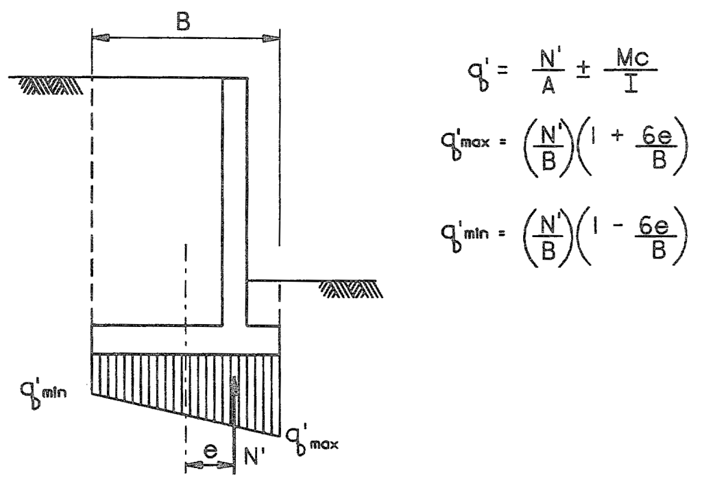
You may recall that, for a uniform pressure distribution, the load is in the middle of the distribution. If a shallow foundation is loaded concentrically, the load is through the centroid, and this is the case. That is designated by the centreline. If the load is concentric, the eccentricity e = 0 and the two pressures q’_min and q’_max are both the same, as we see in the equations above, namely the load divided by the width of the foundation.

If the load is eccentric, e is nonzero. As e increases, q’_max increases and q’_min decreases. When we reach the point where e = B/6, q’_min = 0. Beyond that point we get liftoff from one end of the foundation, which is generally not an acceptable result, especially since foundations cannot transmit tension between the soil and the foundation. As long as -B/6 < e < B/6, both q’_min and q’_max are positive and at least this criterion is met. This region is referred to as the “middle third” and is crucual to the success of shallow foundations.

Eccentricity in loads is not strictly the result of off-centroid loads. It can also be due to a moment on the foundation, in which case e = M/N’ (without any other factors to make the load eccentric.)

As mentioned earlier, this is the simplest case. Things get complicated when we actually implement this concept, and these are discussed in Foundation Design and Analysis: Shallow Foundations, Bearing Capacity II.

General Expression for Trapezoidal Loads

If we look at the diagram above, there’s a similarity between that and the “ramped” loads we see bearing on retaining walls, the result of increasing vertical pressure (and by extension horizontal pressure) on the wall with increasing depth. Traditionally in retaining walls we divide such a ramped load up into a “rectangular” portion (constant) and a “triangular” portion (zero at one end, nonzero at the other.) But in reality we can develop a simple expression that is valid for linearly varying loads with non-negative pressures.

Consider the foundation above. It can be shown that the resultant force on the foundation due to the resisting pressure of the soil is given by the equation

$N' = 1/2\,B\left ({\it q'_{min}}+{\it q'_{max}}\right )$ (1)

or, more simply the average of the end pressures times the length $B$ of the foundation/wall section/beam. It can be shown that, if we define

$p' = \frac{q'_{min}}{q'_{max}}$ (2)

Then the distance from the end with $q'_{min}$ to the location of the resultant is

$x_{tot} = \frac{B}{3}\,{\frac {{\it p'}+2}{{\it p'}+1}}$ (3)

For the case of the triangle load ( $p' = 0$ ) $x_{tot} = \frac{2B}{3}$ and for the uniform load ( $p' = 1$ ) $x_{tot} = \frac{B}{2}$ , as we know. If we subtract the two we get the maximum eccentricity $e_{max} = \frac{B}{6}$ , which we know defines the middle third.

So to not leave out the retaining wall and beam people, let’s consider the following example of sheet pile design using Pile Buck’s SPW911 software.

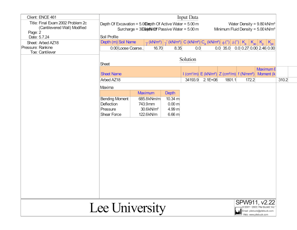
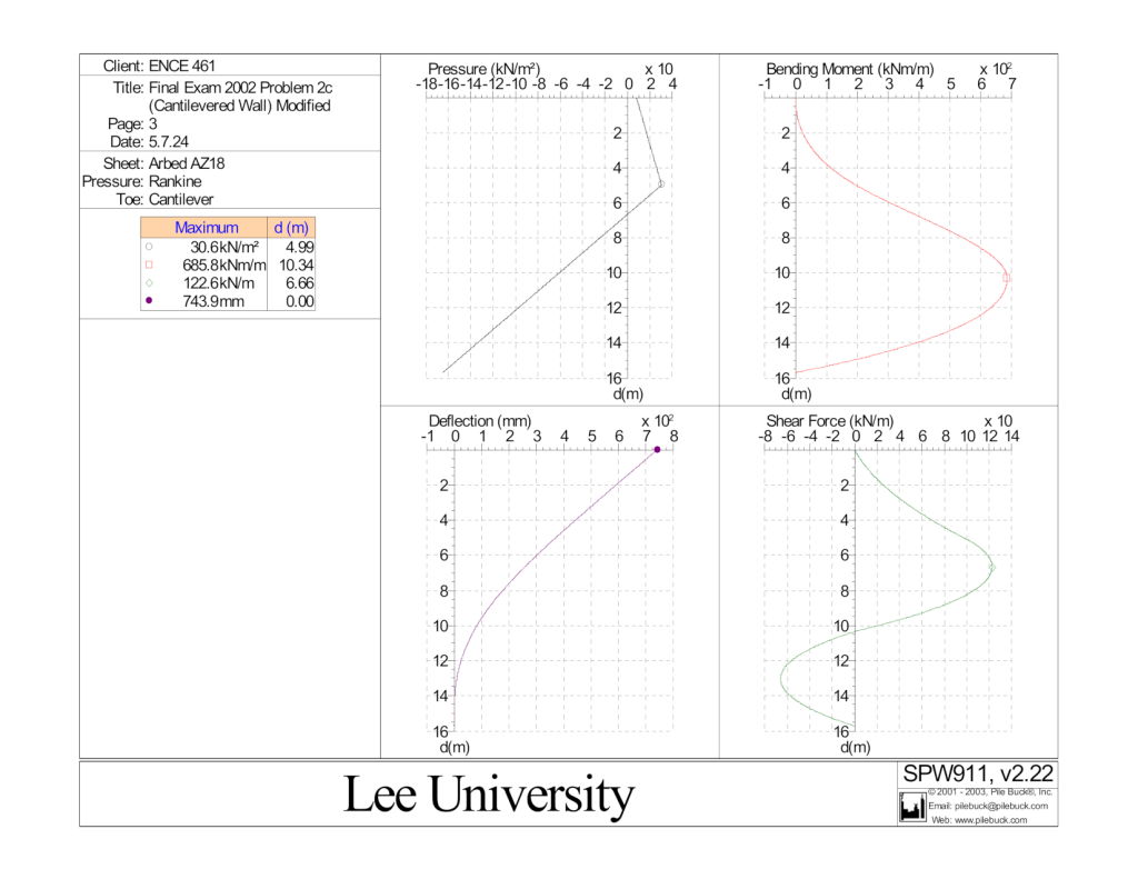
We’ll concentrate on the part which is above the dredge line, a length of 5 m. In this region there is only active pressure on the soil side of the wall; because of the 30 kPa surcharge at the surface, the load has a trapezoidal shape. Without going into the geotechnics of retaining walls (which you can review in the post Foundation Design and Analysis: Retaining Walls, Concrete Gravity Retaining Walls) the lateral pressure at the top of the wall is 8.2 kPa (from the table) and at the dredge line 30.6 kPa (from the main graphic, the maximum pressure.) We can thus say the following:

From Equation (2), adjusting the notation for retaining walls, $p' = \frac{8.2}{30.6} = 0.268$ .
From Equation (3), again adjusting the notation, $x_{tot} = \frac{5}{3} \frac{0.269 + 2}{0.269+1} = 2.98\,m$ from the top of the wall (smaller pressure,) or 2.02 m from the dredge line.
By Equation (1), the magnitude of the resultant $N' = 97 \frac{kN}{m}$ (that’s metre of horizontal wall.) A free-body diagram of the upper 5 m of the wall tells us that, since we’ve replaced a distributed load with a resultant, the shear at the dredge line should be the same. Looking at the table, at 4.97 m from the top, the shear $F = 96.3 \frac{kN}{m}$ , which is very close.
Same free-body diagram shows us that the moment in the sheeting at the dredge line should be the resultant force times the distance from the resultant to the dredge line. Thus the moment $M = (97)(2.02) = 195.94 \frac{kN-m}{m}$ . This too compares favourably with the moment at 4.97 m from the top, which is $M = 193 \frac{kN-m}{m}$

It’s possible to do everything with resultants instead of distributed load integration, but for situations like this it’s easier to do the integration. With numerical methods such as SPW 911 uses, the wall is divided up into finite differences and each difference can be considered a beam, the results summed up and the pressures reduced to resultants. Resultants are very useful for determining boundary conditions like the shear and moment at supports. As noted in this post, if resultants are always used in place of distributed loads, the shears and moments will be conservative, unacceptably so in some cases.