More Uses for p-q Diagrams

In our last post on p-q diagrams we discussed their basic concept and application. In this post we’ll expand on that for two applications: using it to estimate the friction angle and cohesion for multiple triaxial tests, and using it to plot the failure function.

Processing Triaxial Test Results

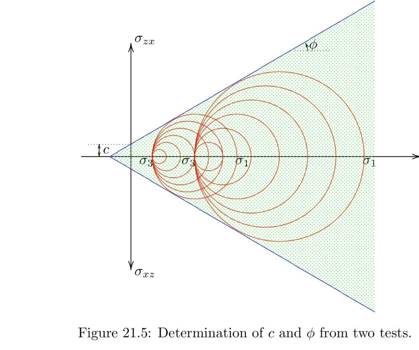
The process of determining internal friction angle and cohesion from successive triaxial tests (i.e., those where the confining stress is successively increased) is well known. In the case of two tests, using the standard $\sigma - \tau$ diagram, the tangent line between the two circles is unique (well, there are two of them, but the slopes and intercepts have opposite signs) as shown below.

Stress Failure Envelope (from Verruijt and van Bars (2007))

If we use the p-q diagram, as we saw earlier, the process is even simpler, as two points have a unique line between them.

But what happens with three tests? Mathematically there is no guarantee of a unique line, and given the nature of geotechnical testing it is the extraordinary lab which could hit such as result. It’s also possible that the failure envelope is non-linear, as shown below.

So is there a way to at least get a decent approximation without guesswork or graphics skills? The answer is “yes” and it involves using p-q diagrams in conjunction with a spreadsheet. The mathematical concept behind this is here and we have an example to show how it is done. The problem is taken from Tchebotarioff’s (1951) classic soil mechanics test. The results of three triaxial tests are as follows, the failure stresses are in tsf:

Test	$\sigma_3$	$\sigma_1$	p	q
1	0.2	0.82	0.51	0.31
2	0.4	1.6	1	0.6
3	0.6	2.44	1.52	0.92

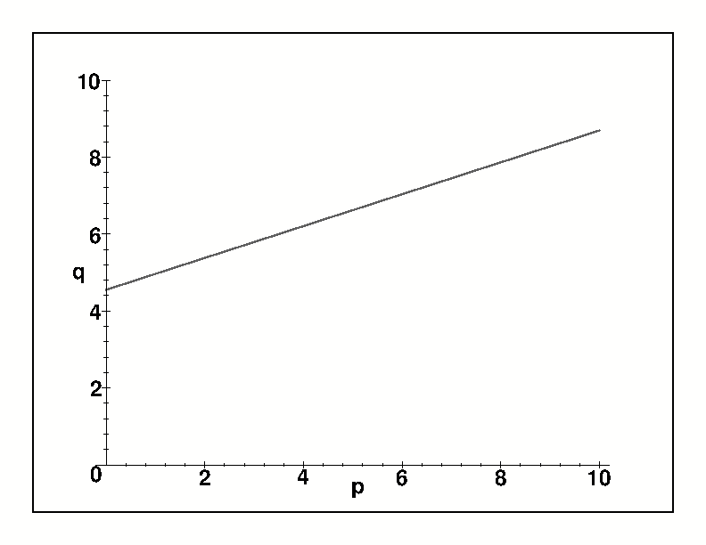
We’ve taken the liberty of computing the p and q values for each test. Now we can plot these in our spreadsheet.

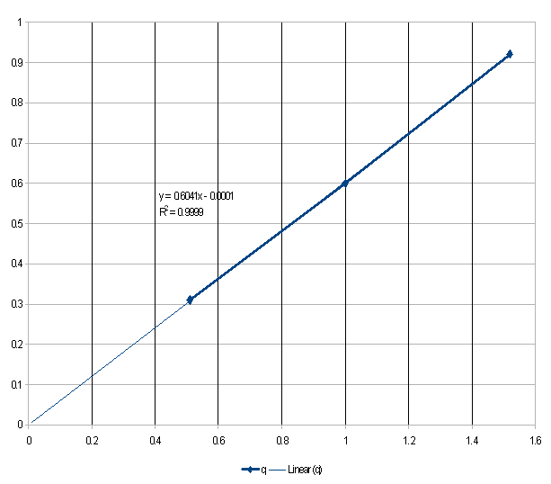
We’ve also taken the liberty to use the spreadsheet’s “trend line” feature to plot a linear “curve fit” for the points. The slope of the equation $m=tan \delta = sin \phi = 0.6041$ , which yields both $\delta = 31.1^\circ$ and $\phi = 37.2^\circ$ . For the intercept $b = c\sqrt {1-\left (\tan(\delta)\right )^{2}} = 0.0001$ , which means we can solve for the cohesion, but in this case the quantity is so small it’s probably best to assume that the cohesion is zero.

The $R^2$ value for this problem is very high, so the correlation is good. We can use this parameter to determine whether we have a good correlation or not. We can also use least-squares trend line analysis for non-linear failure envelopes, although when we consider the “kink” caused by preconsolidation this may not be as meaningful as one would like.

Plotting the Failure Function

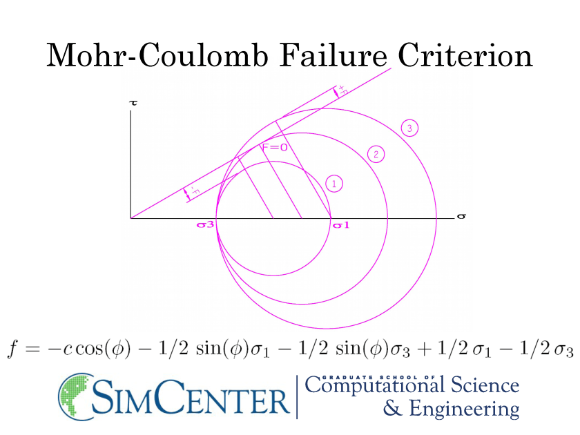
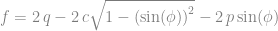
As mentioned earlier, the Mohr-Coulomb failure function is define in this way:

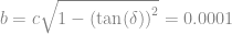
A little math transforms this into

$f=2\,q-2\,c\sqrt {1-\left (\tan(\delta)\right )^{2}}-2\,p\tan(\delta)$

$f=2\,q-2\,c\sqrt {1-\left (\sin(\phi)\right )^{2}}-2\,p\sin(\phi)$

Since $\delta$ and $c$ are known, this suggests that we can plot the failure function three-dimensionally. Consider the case where $\delta = \frac{\pi}{8}$ and $c = 5$ . The p-q diagram for the failure envelope $f = 0$ is shown below.

If we plot the failure function three-dimensionally, we obtain this result:

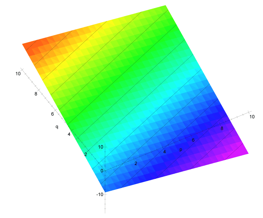
The failure envelope of the previous diagram is the contour line which stops at the q-axis at around q = 4.6. Values below this line are negative and values above it are positive. Positive values of $f$ indicate failure and an illegal stress state. The failure function is used extensively in finite element analyses like this one.